Even More NBA Stats ... but in R no less!: LeBron James's Career PPG (and maybe MJ too)

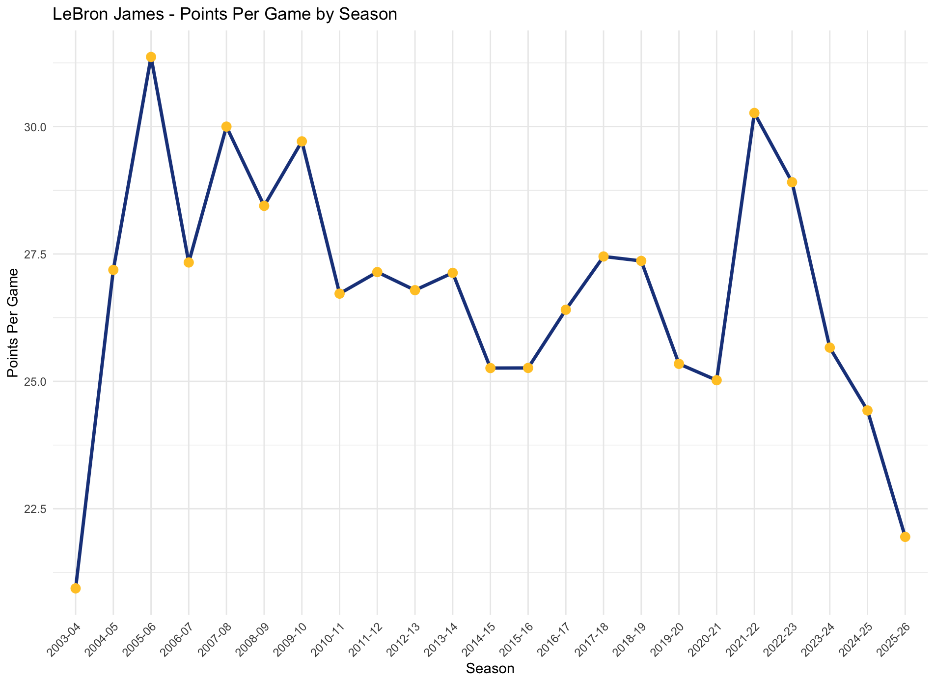
A couple of days ago (January 9, 2026) I watched LeBron and the Lakers take on the Milwaukee Bucks. He played well (26, 9, and 10 is pretty damned good, in fact.) Figures I would use the code from my previous post on Klay Thompson. Here’s what we get (including the more generalized code I promised).

The more generalized code I promised first:


# Install packages (only need to do this once)
install.packages("hoopR")
install.packages("ggplot2")
install.packages("dplyr")

# Load packages
library(hoopR)
library(ggplot2)
library(dplyr)

# ===== CONFIGURATION - CHANGE THIS FOR DIFFERENT PLAYERS =====
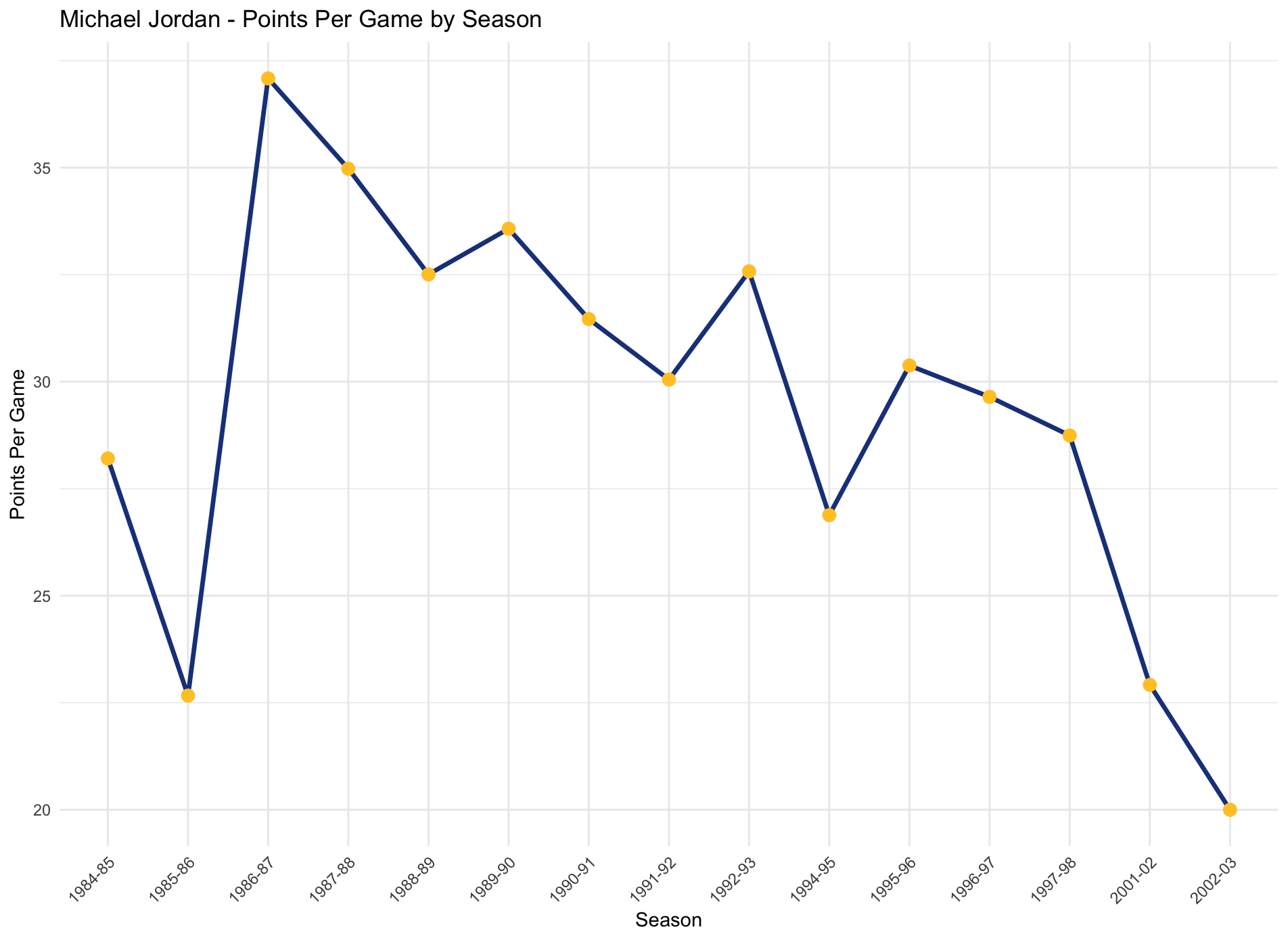
player_name <- "Michael Jordan"  # Change this to any player
# ===============================================================

# Get player ID
players_list <- nba_commonallplayers(season = "2024-25")
players <- players_list$CommonAllPlayers

player_id <- players %>% 
  filter(DISPLAY_FIRST_LAST == player_name) %>% 
  pull(PERSON_ID)

print(paste(player_name, "ID:", player_id))

# ===== PLOT 1: Annual Averages =====

# Get career stats by season
player_career <- nba_playercareerstats(player_id = player_id)

# Extract the season totals dataframe and convert to numeric
player_seasons <- player_career$SeasonTotalsRegularSeason %>%
  mutate(
    PTS = as.numeric(PTS),
    GP = as.numeric(GP),
    PPG = PTS / GP
  )

# Create the annual averages plot
plot1 <- ggplot(player_seasons, aes(x = SEASON_ID, y = PPG)) +
  geom_line(group = 1, color = "#1D428A", linewidth = 1.2) +
  geom_point(color = "#FFC72C", size = 3) +
  theme_minimal() +
  labs(title = paste(player_name, "- Points Per Game by Season"),
       x = "Season",
       y = "Points Per Game") +
  theme(axis.text.x = element_text(angle = 45, hjust = 1))

print(plot1)

# Save Plot 1
ggsave(paste0(gsub(" ", "_", tolower(player_name)), "_ppg_by_season.png"), 
       plot = plot1, width = 10, height = 6, dpi = 300)


# ===== PLOT 2 & 3: Game-by-Game Scatterplots =====

# Get unique seasons from career stats
seasons_list <- unique(player_seasons$SEASON_ID)

all_games <- list()

for(s in seasons_list) {
  tryCatch({
    game_log <- nba_playergamelog(player_id = player_id, season = s)
    
    # Extract the dataframe from the list
    if("PlayerGameLog" %in% names(game_log)) {
      all_games[[s]] <- game_log$PlayerGameLog
    } else {
      all_games[[s]] <- game_log
    }
    
    print(paste("Got data for", s))
    Sys.sleep(0.5)  # Small delay to avoid rate limiting
  }, error = function(e) {
    print(paste("Error with season", s, ":", e$message))
  })
}

# Combine all games
player_games <- bind_rows(all_games) %>%
  mutate(
    PTS = as.numeric(PTS),
    GAME_DATE = as.Date(GAME_DATE, format = "%b %d, %Y")
  )

# DEBUG: Let's look at a sample of MATCHUP values
print("Sample MATCHUP values:")
print(head(unique(player_games$MATCHUP), 20))

# Extract team abbreviation from MATCHUP (first 3 characters before space, @, or vs.)
player_games <- player_games %>%
  mutate(
    Team_Abbrev = gsub("^([A-Z]{2,3}).*", "\\1", MATCHUP)
  )

# DEBUG: Check what team abbreviations we're getting
print("Unique team abbreviations found:")
print(unique(player_games$Team_Abbrev))

# Get unique teams and map to full names
team_mapping <- data.frame(
  abbrev = c("CLE", "MIA", "LAL", "GSW", "DAL", "BOS", "PHX", "DEN", "MIL", 
             "PHI", "TOR", "BKN", "CHI", "ATL", "WAS", "ORL", "CHA", "DET",
             "IND", "NYK", "MEM", "MIN", "NOP", "OKC", "POR", "SAC", "SAS",
             "UTA", "LAC", "HOU"),
  full_name = c("Cavaliers", "Heat", "Lakers", "Warriors", "Mavericks", "Celtics",
                "Suns", "Nuggets", "Bucks", "76ers", "Raptors", "Nets", "Bulls",
                "Hawks", "Wizards", "Magic", "Hornets", "Pistons", "Pacers",
                "Knicks", "Grizzlies", "Timberwolves", "Pelicans", "Thunder",
                "Trail Blazers", "Kings", "Spurs", "Jazz", "Clippers", "Rockets")
)

# Map abbreviations to full names
player_games <- player_games %>%
  left_join(team_mapping, by = c("Team_Abbrev" = "abbrev")) %>%
  mutate(Team = ifelse(is.na(full_name), Team_Abbrev, full_name))

# Get the unique teams the player actually played for (in chronological order)
unique_teams <- player_games %>%
  group_by(Team) %>%
  summarize(first_game = min(GAME_DATE), n_games = n()) %>%
  arrange(first_game)

print("Teams and game counts:")
print(unique_teams)

# Filter to only teams with significant number of games (likely >10 games means they actually played there)
actual_teams <- unique_teams %>%
  filter(n_games > 10) %>%
  pull(Team)

print(paste("Teams actually played for (>10 games):", paste(actual_teams, collapse = ", ")))

# Filter player_games to only include actual teams
player_games <- player_games %>%
  filter(Team %in% actual_teams)

# Create a color palette
team_colors <- c("#E69F00", "#56B4E9", "#009E73", "#F0E442", "#0072B2", 
                 "#D55E00", "#CC79A7", "#999999", "#000000", "#E6AB02")

# Assign colors to teams
team_color_map <- setNames(team_colors[1:length(actual_teams)], actual_teams)

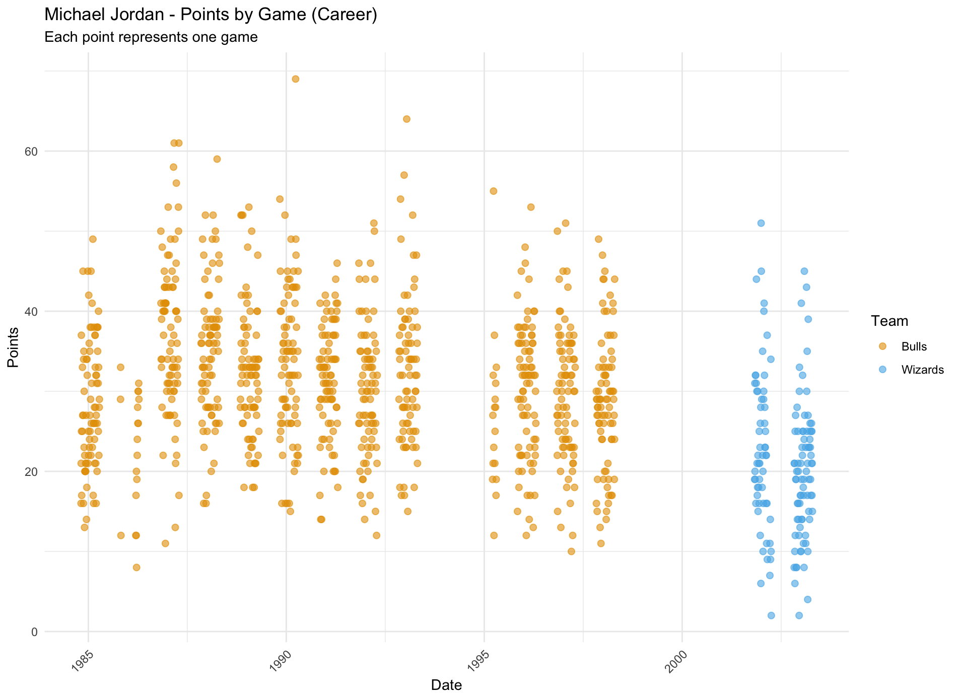
# Create scatterplot WITHOUT regression line
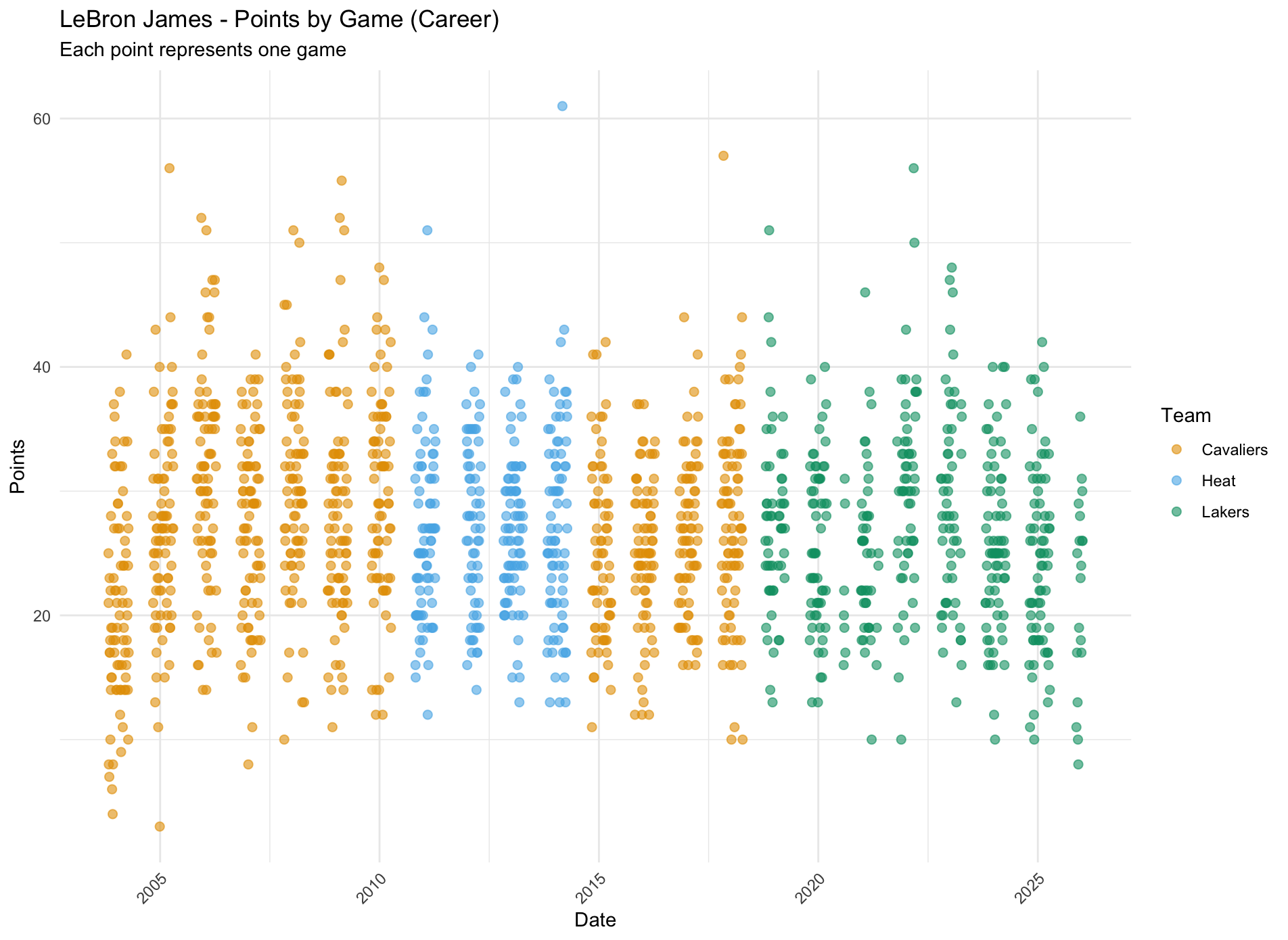
plot2 <- ggplot(player_games, aes(x = GAME_DATE, y = PTS, color = Team)) +
  geom_point(alpha = 0.6, size = 2) +
  scale_color_manual(values = team_color_map) +
  theme_minimal() +
  labs(title = paste(player_name, "- Points by Game (Career)"),
       x = "Date",
       y = "Points",
       subtitle = "Each point represents one game",
       color = "Team") +
  theme(axis.text.x = element_text(angle = 45, hjust = 1))

print(plot2)

# Save Plot 2
ggsave(paste0(gsub(" ", "_", tolower(player_name)), "_points_by_game_no_regression.png"), 
       plot = plot2, width = 12, height = 6, dpi = 300)


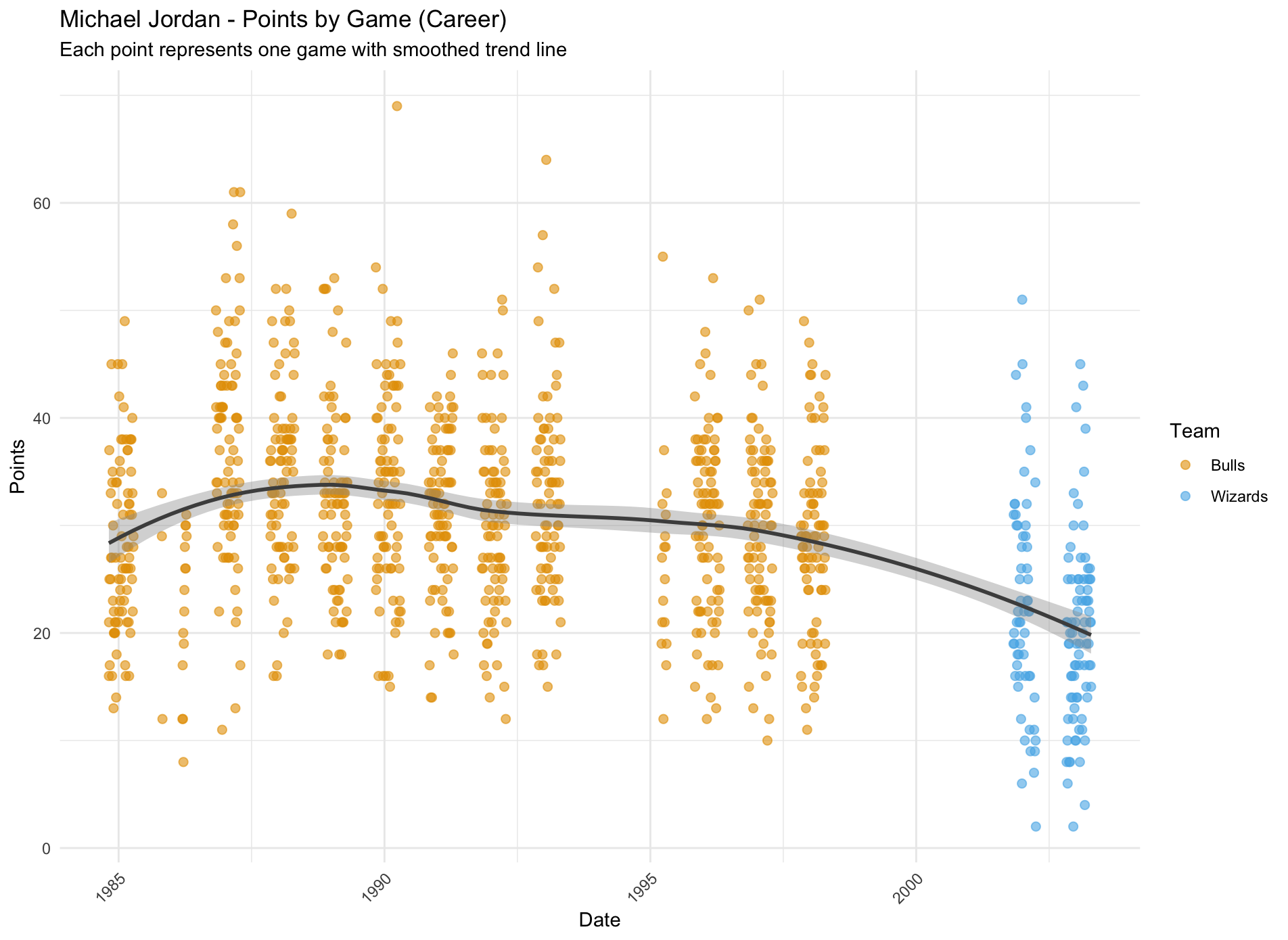
# Create scatterplot WITH regression line
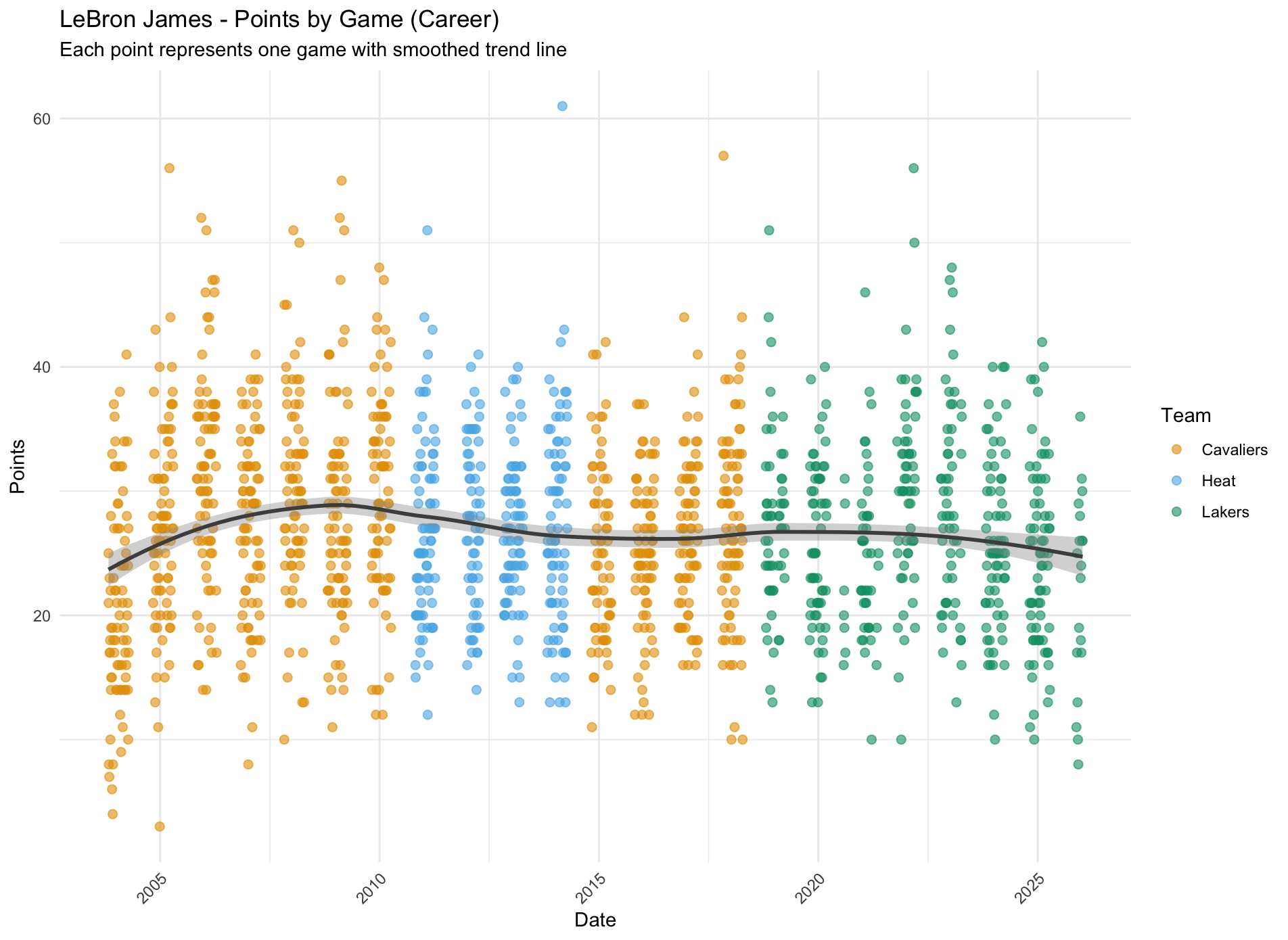
plot3 <- ggplot(player_games, aes(x = GAME_DATE, y = PTS, color = Team)) +
  geom_point(alpha = 0.6, size = 2) +
  geom_smooth(aes(group = 1), method = "loess", color = "gray30", se = TRUE) +
  scale_color_manual(values = team_color_map) +
  theme_minimal() +
  labs(title = paste(player_name, "- Points by Game (Career)"),
       x = "Date",
       y = "Points",
       subtitle = "Each point represents one game with smoothed trend line",
       color = "Team") +
  theme(axis.text.x = element_text(angle = 45, hjust = 1))

print(plot3)

# Save Plot 3
ggsave(paste0(gsub(" ", "_", tolower(player_name)), "_points_by_game_with_regression.png"), 
       plot = plot3, width = 12, height = 6, dpi = 300)

print("All three plots saved successfully!")

Plots second (for LeBron James in this iteration):

LeBron PPG Over His Career