3 minutes
Going For It on 4th Down!
Introductory Setup
This past Thanksgiving I headed over to Sioux City, IA to visit my folks, brother, sister-in-law, and baby sister. Thursday found my father and I watching the Chiefs game against the Cowboys (Dallas carried the day 31-28). At some point, my dad turned to me and said something to the effect of you, “Doesn’t it seem like teams nowadays are going for it on fourth down far more than they used to?” “Oooh, I suppose so, though that’s a fantastically empirical question we could figure out.” “Sounds like a question for ChatGPT,” he comically quipped. As per usual, I told him that don’t sound like any fun and said I’d much rather code it up myself. So, here, below, is the workflow to investigate (github repo with everything is available here). I’ve split said repo into a number of different steps, which we’ll have a look at below.
Step 1: Gathering the Data
As always, we start by gathering the data we need. Obviously we need a way to pull down some NFL stats—and the nflreadpy library is designed exactly for this. So our first step is to create a script to download the NFL data required.
Here’s our data fetching script—I also thought I would try working with polars rather than my/our usual pandas. (Polars touts itself as blazingly fast—since we’re looking at quite a lot of data [twenty plus years of play by play data], I figured I’d give it a try. I also wrote some miscellaneous scripts to benchmark polars vs. pandas and, indeed, the former is faster.)
import nflreadpy as nfl
import polars as pl

def fetch_pbp_data(years: list[int]) -> pl.DataFrame:
    """
    Fetch and combine play-by-play data for given years using the nflreadpy library.
    """
    print(f"Fetching data for years: {years}")
    # nflreadpy concatenates automatically if you pass a list
    pbp = nfl.load_pbp(seasons=years)
    print(f"Loaded {len(pbp)} plays")
    return pbp

if __name__ == "__main__":
    # Example: 2000 to 2025
    years = list(range(2000, 2026))
    df = fetch_pbp_data(years)
    df.write_parquet("data/pbp_raw.parquet")  # We'll write this to parquet.
Step 2: Processing the Data
Now that we’ve got all the data into a nice .csv file, we can filter out the fourth down data we are interested in. Step 2 does just that:
import polars as pl

def load_pbp() -> pl.DataFrame:
    return pl.read_parquet("data/pbp_raw.parquet")

def filter_fourth_down_attempts(df: pl.DataFrame) -> pl.DataFrame:
    fourth_downs = df.filter(pl.col('down') == 4.0)

    attempts = fourth_downs.filter(pl.col('play_type').is_in(['pass', 'run']))

    attempts = attempts.with_columns(
        (pl.col('fourth_down_converted') == 1).alias('converted')
    )

    return attempts

def aggregate_season_attempts(attempts: pl.DataFrame) -> pl.DataFrame:
    # Unique games per season (each game appears once, but two teams play)
    games_per_season = attempts.group_by('season').agg(pl.col('game_id').n_unique() * 2)

    season_stats = attempts.group_by('season').agg(
        total_attempts = pl.col('play_id').count(),
        total_converted = pl.col('converted').sum(),
        total_team_games = pl.col('game_id').n_unique() * 2  # each game = 2 team-games
    ).join(games_per_season, on='season', how='left')

    season_stats = season_stats.with_columns(
        (pl.col('total_attempts') / pl.col('total_team_games')).alias('attempts_per_game'),
        (pl.col('total_converted') / pl.col('total_attempts')).alias('conversion_rate')
    )

    return season_stats

if __name__ == "__main__":
    df = load_pbp()
    attempts = filter_fourth_down_attempts(df)
    season_trends = aggregate_season_attempts(attempts)
    season_trends.write_csv("data/season_fourth_down_trends.csv")
    print(season_trends)
Steps 3-8: Visualizing the Data
With everything cleaned and filtered we can produce some plots. I’ll just put the plots here and point again to the github repo that has separate scripts for all these visualizations.
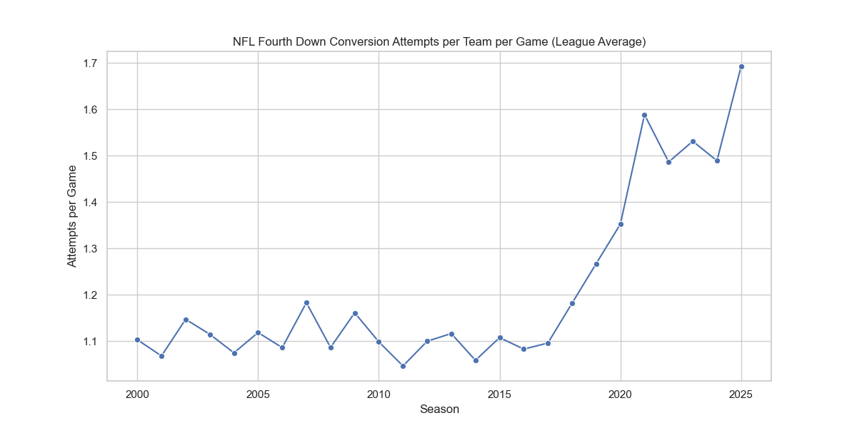
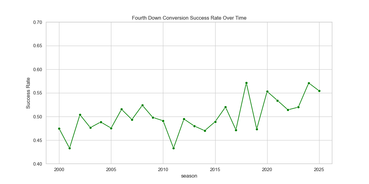
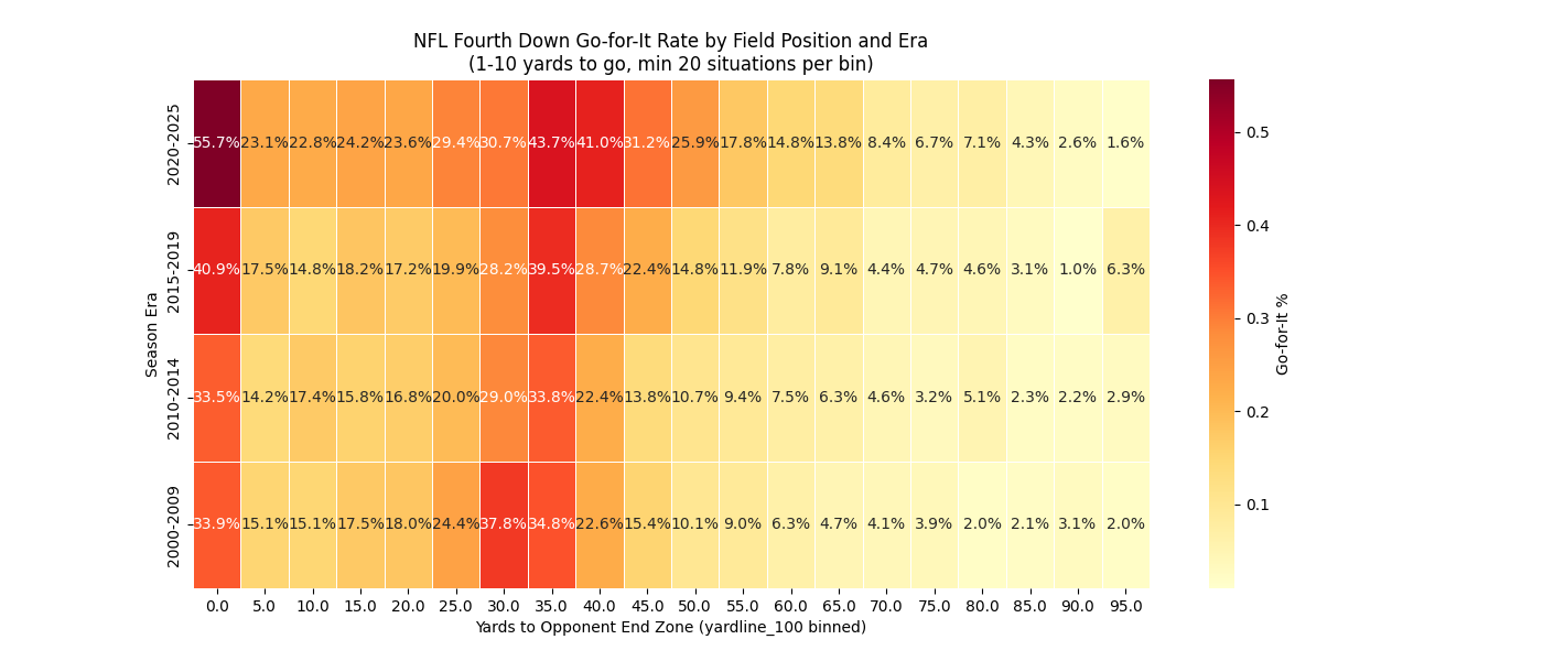
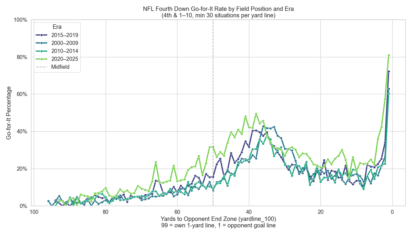
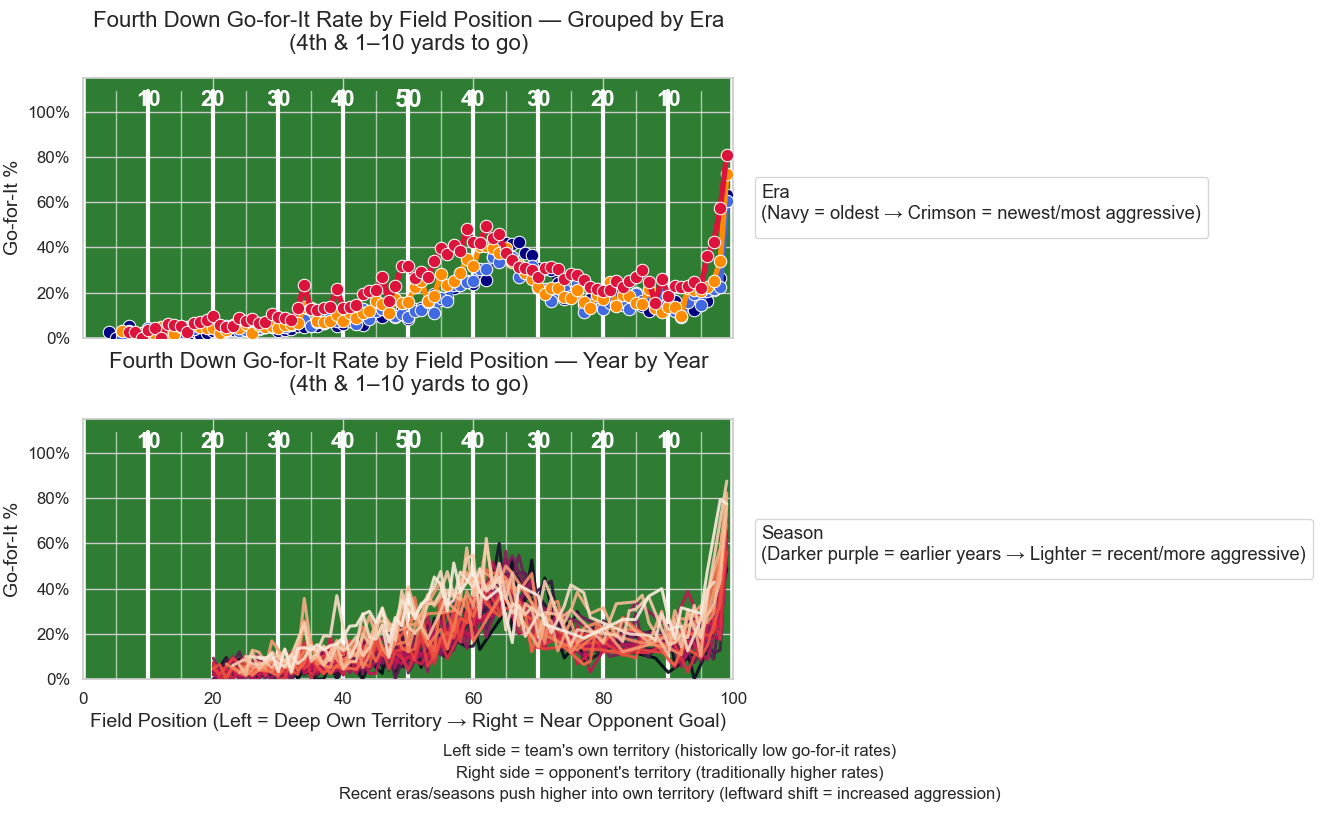
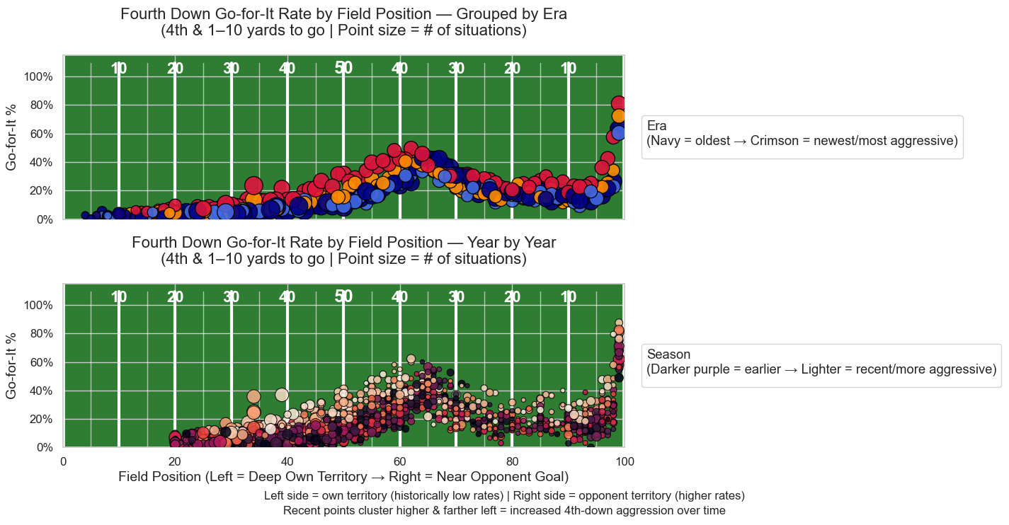
Obviously, there are some tweaks we could make to the aesthetics of many of these to fine-tune them even further. More to come, as always.
python data parsing data extraction data analysis NFL python for sports polars matplotlib data visualization csv nflreadpy
536 Words
2026-01-09 00:01