Fitzgerald … Hemingway … Steinbeck

Lately I have been spending a fair amount of time working on my portfolio for the required “Post_Tenure Review” at my current institution. I spent quite a bit of time canvassing a great deal of the DH/computer programming learning I have acquired over the last couple of years. I gave a somewhat interesting test project version of some more stylometry/text classification work,¹ focusing quite directly on some work another (former) student of mine, William Mastin, and I have been doing on one of his most favorite authors, Ernest Hemingway. It would be absolutely impossible to canvas the interminable discussions we had about “Papa” as of late, but I figured I could just share some of the computational work that was tangentially related to this endeavor.

I think the real impetus for much of this computational investigation was due to the fact that, in many of those conversations, William would often draw parallels and comparisons between Hemingway and Fitzgerald (we even read very closely one of my most favorite Fitzgerald stories, “Babylon Revisited”). I was curious—could one, say, train a machine learning model to tell the difference between a text written by Hemingway and one by Fitzgerald? For sure—and what I still find so fascinating about all of this is that the way in which the models can do this are not really all that “complex” or “complicated” or “sophisticated”—at least, they are definitely not more sophisticated than when a seasoned reader can (perhaps somewhat) intuitively tell the difference immediately between Hemingway’s and Fitzgerald’s stylistic tendencies. So let’s write a little Python code and I’ll try to take readers through what’s going on along each step of the process.²

The first step is data gathering, so we head over to Project Gutenberg.org to grab texts that are available and in the public domain by both Fitzgerald and Hemingway.³ Once we have some texts that we can use to train and test the classifier models, we can start coding. We will be utilizing one of the go-to machine learning libraries within Python, sci-kit learn, an absolute staple for those working in machine learning. Thus we start with our import statements (we’re also using seaborn and matplotlib again for plotting, pandas for data wrangling, etc. [the load_data function is just a simple function to read in all the text files and keep track of the author of each text]):

from helper_functions import load_data
import os
import seaborn as sns
import matplotlib.pyplot as plt
import pandas as pd
from sklearn.naive_bayes import MultinomialNB
from sklearn.feature_extraction.text import CountVectorizer
from sklearn.model_selection import train_test_split
from sklearn.metrics import classification_report, confusion_matrix, accuracy_score
import spacy
nlp = spacy.load('en_core_web_lg')

Next we call our load data function to load in all of our text files and then convert that into a pandas DataFrame that contains the text of the work (in the text_data column) along with the named author in the label column. We also want to let sklearn know which columns have the “text” and which one contains the “real/true” labels for each text:

text_data, labels = load_data('data')
df = pd.DataFrame(list(zip(text_data, labels)), columns=['text_data', 'label'])

X = df['text_data']
y = df['label']

Then we utilize one of the functions from the sklearn library that takes the dataset and splits it into “training” and “testing” sets. The training set will be the data that the model is given to “learn” what makes a Hemingway text a Hemingway text (and similarly for Fitzgerald); the “testing” data is just that: those are the texts that the model has never seen before and thus will make predictions on/about. The normal split in machine learning is usually 80% of the data used for training and 20% for testing, but here we’re passing a percentage of 30%:

X_train, X_test, y_train, y_test = train_test_split(
													X,
													y,
													test_size=0.3,
													random_state=42)

Now that the training and testing sets are split up, we can start to transform all of this text data into what the model can understand, namely, numbers:

# Create a bag-of-words representation of the text data
vectorizer = CountVectorizer(stop_words='english')
X_train_vec = vectorizer.fit_transform(X_train)
X_test_vec = vectorizer.transform(X_test)

As seasoned DH folks knows, what the CountVectorizer() function does is it takes all of the words in the text and converts the whole text file into just a long list of words. (This is often called a “bag of words” representation because all the program is doing is, quite literally, counting each word and how many times each word appears; everything ends up in a “bag” because this process disregards grammar and also word order too.) The second and third lines of code just apply this technique/function to both the training and testing sets—for more information, the .fit method is explained in the documentation here and the .fit_transform here.

Once the text files are converted into a matrix (i.e. the data has been “vectorized”), one can then train a model to make predictions on the testing data. For this little project, we’ll utilize a widely used algorithm that is based on “Bayes’ theorem,” which “describes the probability of an event, based on prior knowledge of conditions that might be related to the event.”⁴ This is a very commonly used model for “text classification” problems and it thus serves our purposes here well enough.⁵ Once the model is instantiated, we can fit it on our data as follows:

nb = MultinomialNB()
nb.fit(X_train_vec, y_train)

So how accurate is the model on the texts that were set aside for the testing purposes? One of the standard ways to see the accuracy of the model is to use a number of metrics—i.e. “precision,” “recall,” “f1-score,” etc.⁶ Sklearn has a built-in function for this, classification_report which quickly provides us with these metrics and scores. Below we’ll print out the accuracy_score for the testing data along with the other metrics:

# Evaluate the model on the testing set
accuracy = nb.score(X_test_vec, y_test)
print(f"The accuracy score for this NaiveBayes Classifier is: {accuracy}")

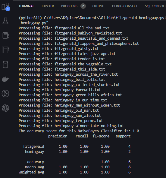
These are fantastic scores for the model. Of course, there are also nice and simple ways to visualize the predictions the model has made by utilizing what is called a “confusion matrix”. This is a simple picture that shows us the number of “true positives,” “true negatives,” “false positives,” and “false negatives.” The code to produce the plot is, again, rather simple enough to implement:

# Predict the class labels for the test set
y_pred = nb.predict(X_test_vec)

# Compute the confusion matrix
cm = confusion_matrix(y_test, y_pred)

# create a list of class labels
classes = ['fitzgerald', 'hemingway']

# plot the confusion matrix
sns.heatmap(cm,
			annot=True,
			fmt='d',
			cmap='viridis',
			xticklabels=classes, yticklabels=classes)

# add axis labels and title
plt.xlabel('Predicted Label')
plt.ylabel('True Label')
plt.title('Confusion Matrix')
plt.show()

The plot produced looks as follows:

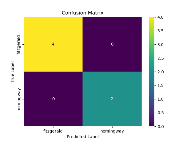
A classifier with scores like these is considered to be performing extremely well. But what if we wanted to kick the tires on this model just a little bit more by passing it, say, a text by Hemingway that the model has never before encountered, either in training or testing (many machine learning modeling workflows include this as the “validation” set, a sample to make a prediction on that was not in the training or testing datasets)? Well, let’s feed this brand-new (to the model) text and see who it predicts wrote it. We’ll ask it to make a prediction about Hemingway’s “The Snows of Kilimanjaro.” Again, easy enough—and the steps are the same (we read in the text file, vectorize it, and then pass it to the model to make a prediction):

# Define a new text sample to classify—Hemingway's "The Snows of
# Kilimanjaro"
with open(r'test_data\hemingway_snows.txt') as f:
    new_text =  f.read()  

# Transform the new text sample into a bag-of-words representation
new_counts = vectorizer.transform([new_text])

# Use the trained model to predict the label of the new text sample
new_pred = nb.predict(new_counts)

# Print the predicted label
if new_pred == 1:
    print("The model predicts that this text is by Hemingway ...")
else:
    print("The model predicts that this text is by Fitzgerald ...")

This code outputs the following:

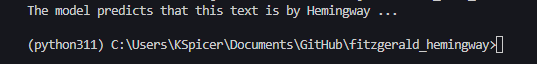
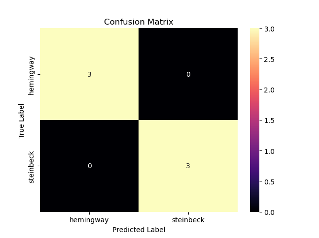
Nice—a perfectly correct prediction. I should say that one could easily wonder just a bit if the binary parameter here in this problem—a text is either by Hemingway or it’s not—does come with some starting assumptions that one could tweak slightly if they wanted. What if the comparison was not between Hemingway and Fitzgerald but between Hemingway and someone a reader might consider to already be somewhat “closer” to Hemingway in terms of style? What about texts by John Steinbeck? Again, we can reuse the code already and simply alter it so that we have the program read in the texts by Steinbeck in the training part of the process. Once again, a very simple Naive Bayes classifier can quite easily distinguish between Hemingway and Steinbeck too:

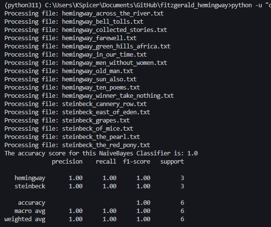
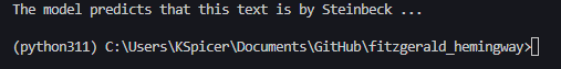
And, once more, if we pass it a text by Steinbeck (In Dubious Battle) for validation, we can ask for another prediction—and we get:

What I find so curious about this entire process is what I mentioned earlier, the model can seem to figure out who authored what simply by counting words and keeping track of their frequencies—nothing more sophisticated would seem to be required here. There are, of course, far more intricate algorithms and vectorizers that can be used when working with textual data (the “term-frequency inverse document frequency,” TF-IDF for short, is just one example), but such sophistication seems unnecessary—at least here in this particular case. The frequency counts of words seem to be enough to distinguish between the writing of these authors. It might perhaps go without saying, but I think these developments ask those of us working within the humanities to potentially rethink how we want to talk about something like a writer’s “style.” Those working in literature might love to use all kinds of literary techniques, rhetorical tropes, and much more to discuss a writer’s style. The machine would seem to be able to get along just fine by merely(?) counting things. As I say, I think this is incredibly thought-provoking for humanistic study more broadly—and I continue to be amazed with the results.