6 minutes
Training a SpaCy Text Classifier on Supreme Court Opinions: Classifying Opinions by Century
Continuing some work with the Supreme Court databases I’ve been fiddling around with lately, I was wondering if I could get a machine learning model to be able to correctly identify and classify a Supreme Court opinion by the decade in which it was written. So let’s grab some data and see what we can do!
There is a really wonderful github repo that contains the .json files of all the Supreme Court cases made available through the CourtListener API. I forked this repo and then proceeded to do some basic data gathering/wrangling (all the code for the data wrangling and exploratory data analysis (EDA) are available in the the repo folder here) First, our libraries:
import json
import os
from pathlib import Path
import pandas as pd
from sklearn.model_selection import train_test_split
import spacy
from spacy.util import minibatch
from spacy.training.example import Example
nlp = spacy.blank('en')
All of the files are split up into folders by the century and then with subfolders by year. We can thus write a simple function to grab all these files and get them—as usual—into a dataframe:
def read_jsons_into_dataframe(directory):
    temp_list_of_dfs = []
    directory = directory
    pathlist = Path(directory).rglob('*.json')
    for path in pathlist:
        with open(path) as f:
            json_data = pd.json_normalize(json.loads(f.read()))
        temp_list_of_dfs.append(json_data)
    combined_df = pd.concat(temp_list_of_dfs, ignore_index=True)
    return(combined_df)
Simple enough, we can then just call this function on all of the different century-named folders:
df_1700s = read_jsons_into_dataframe('1700s)
After we do that for all four our centuries, we can just merge them all into one dataframe (oh—and after each of the four were read in we added a label column that had the century in it):
merged_df = pd.concat([df_1700s, df_1800s, df_1900s, df_2000s])
This gives us a nice dataframe with a shape of (63347, 42). Each of the CourtListener files has columns for the plain_text of the case along with other columns that give us the same information in HTML: html and html_with_citations. We also need to create a label column that will store the century the case was written.
After some text cleaning using some of standard data cleaning functions, we could do a little teeny-tiny bit of exploratory EDA on our cleaned-up data:
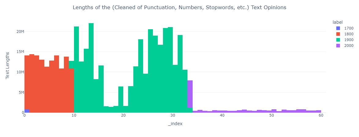
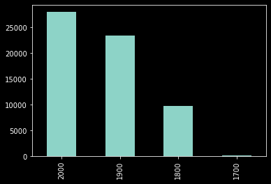
Now, we do have a really sizable data imbalance—we have a ton more examples from the 1800s-2000s than we do from the 1700s. The way I decided to handle this was to simply sample the same number of documents from the 1800s, 1900s, and 2000s that we have for the 1700s—i.e. 135.
Next we can take all our cleaned-up opinions in our file and separate out the texts and the labels and then process them with spaCy using the nlp function (more information on and documentation about spaCy’s TextCategorizer pipeline is available here). We’ll write a simple little function to handle everything as follows:
def make_docs(data, target_file, cats):
    docs = DocBin()
    for doc, label in tqdm(nlp.pipe(data, as_tuples=True, disable=['tagger', 'parser', 'attribute_ruler', 'lemmatizer']), total=len(data)):
        for cat in cats:
            doc.cats[cat] = 1 if cat == label else 0
        docs.add(doc)
    docs.to_disk(target_file)
    return docs
With this function, we can then get tinker just slightly with our main dataframe to get everything ready to be fed to the make_docs function above:
df = pd.read_json('training_json_file.json', orient='records', encoding='utf-8')

# Sanity check here just make sure everything looks good in the dataframe:
print(df.head())

df['text'] = df['cleaned_html'].replace(r'\n',' ', regex=True)
df['label'] = df['label'].astype('str')

# Here we're randomly sampling only 135 texts from each label:
resampled_df = df.groupby('label').apply(lambda x: x.sample(135)).reset_index(drop=True)

# Once again, just a quick sanity check of the labels for each text opinion:
cats = resampled_df.label.unique().tolist()
print(cats)
Everything looks good so we can use sklearn’s train_test_split function to split our data into training and testing sets:
X_train, X_valid, y_train, y_valid = train_test_split(resampled_df["text"].values, resampled_df["label"].values, test_size=0.3)
Let’s see what happens when we feed it a text the model hasn’t seen before. Given that the bulk_scotus repo only goes up to 2015, why don’t we give it a much more recent opinion? (The two recent texts are in the texts_for_testing for the main repo.) We’ll read ’em and see what the model thinks:
tqdm(make_docs(list(zip(X_train, y_train)), "train.spacy", cats=cats))
tqdm(make_docs(list(zip(X_valid, y_valid)), "valid.spacy", cats=cats))
print("Finished making all the docs!")
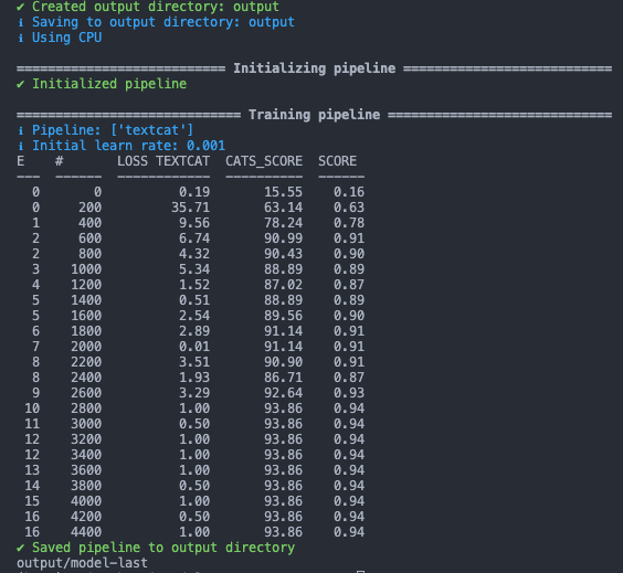
Using a very simple little python script, we can set the model training—the results of which look like the following:
Now we want to do some evaluating of the classifier model we’ve created. I selected out a number of different opinions from each of the four centuries and ran them through the model (the full notebook is available here). One could easily clean-up the output here a little bit to make things easier to read—the model outputs numbers for each of the four classes, with a score 1.0 being a high likelihood that the opinion was from that century:
{'1764_84587':
    {'1700': 1.0,
    '1800': 7.777257948760052e-09,
    '1900': 2.8018092301806703e-16,
    '2000': 9.425196398636101e-20},
'1783_84599':
    {'1700': 0.32349979877471924,
    '1800': 0.034033384174108505,
    '1900': 0.16195958852767944,
    '2000': 0.4805071949958801},
'1944_103915':
    {'1700': 0.0,
    '1800': 0.0,
    '1900': 1.0,
    '2000': 0.0},
'1880_90030':
    {'1700': 0.0,
    '1800': 1.0,
    '1900': 0.0,
    '2000': 0.0},
'1850_86508':
    {'1700': 1.708175368559873e-25,
    '1800': 1.0,
    '1900': 0.0,
    '2000': 0.0},
'1764_84586':
    {'1700': 0.9460902810096741,
    '1800': 0.0035104146227240562,
    '1900': 0.021581759676337242,
    '2000': 0.028817567974328995},
'1985_111301':
    {'1700': 0.0,
    '1800': 0.0,
    '1900': 1.0,
    '2000': 0.0},
'2022_opinion_2':
    {'1700': 5.568387912354698e-38,
    '1800': 5.690646799485532e-28,
    '1900': 1.0,
    '2000': 3.485777328789978e-31},
'1865_87621':
    {'1700': 2.6655867259250954e-05,
    '1800': 0.9999731779098511,
    '1900': 7.38305203640266e-08,
    '2000': 5.533585308720168e-12},
'1902_95542':
    {'1700': 3.664196701011874e-18,
    '1800': 1.0,
    '1900': 5.649902491268908e-18,
    '2000': 3.246556751151545e-34},
'1764_2381788':
    {'1700': 0.384422242641449,
    '1800': 0.038189876824617386,
    '1900': 0.2620941698551178,
    '2000': 0.31529369950294495},
'1920_99495':
    {'1700': 0.0,
    '1800': 4.156211399347631e-12,
    '1900': 1.0,
    '2000': 6.179726227672443e-43},
'1898_94785':
    {'1700': 5.021724189773055e-15,
    '1800': 1.0,
    '1900': 7.398553538091516e-17,
    '2000': 1.226735308388623e-24},
'1783_84600':
    {'1700': 1.0,
    '1800': 9.028870096017272e-09,
    '1900': 1.044657360615986e-09,
    '2000': 5.815799231090324e-11},
'1963_106601':
    {'1700': 0.0,
    '1800': 0.0,
    '1900': 1.0,
    '2000': 0.0},
'2022_opinion_1':
    {'1700': 2.396220373995437e-43,
    '1800': 2.923387118178614e-29,
    '1900': 1.0,
    '2000': 7.380723387276827e-21},
'1804_84713':
    {'1700': 3.133987236392244e-10,
    '1800': 1.0,
    '1900': 0.0,
    '2000': 0.0}}
Actually, there’s a nice little library available through pip that takes a dataframe and export it as a .png (see docs for dataframe-image here):
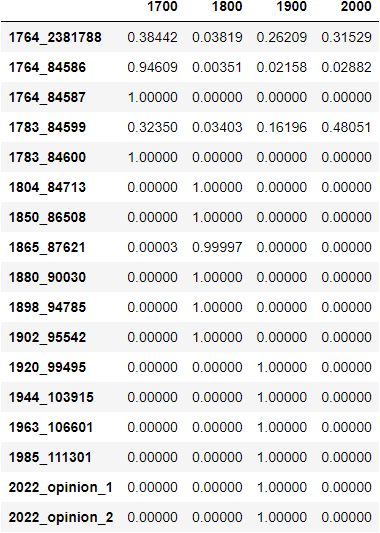
That looks much nicer and way easier to read.
The model correctly classified 76% of the opinions correctly—13 out of 17. Not bad, I suppose. It would be interesting to see what would happen if we didn’t deal with the data imbalance problem and simply fed it the 135 samples from the 1700s along with the full data from the 1800s, 1900s, and 2000s. Sounds like a nice little thing to check out when I get some more free time here.
More to come, as always, I’m sure.
[Update as of Thursday, October 20th, 2022: Increasing the number of samples from the 1800s, 1900s, and 2000s did not result in any increase in terms of accuracy—still 13 out of 17.]
python spaCy spaCy TextClassifier text classification digital humanities dh pandas machine learning data wrangling data cleaning json data
1073 Words
2022-10-17 00:01 (Last updated: 2022-10-20 11:16)