7 minutes
Topic Modeling the United States Supreme Court Utilizing the Top2Vec Library
Here in this post I’d like to continue working on the same project used in the previous post (here) while trying out the Top2Vec library). As is so often the case, I came across this library via Dr. William Mattingly’s YoutTube channel, who devoted two different videos to using this library (here and here). So let’s jump in and see what we can do with this library.
This time around we’re using a slightly different dataset that comes Kaggle—it contains all of the USSC opinions from 1970 on. So let’s load up some libraries and get everything read in as usual. Top2Vec needs a list of strings to process and vectorize, so we’ll convert the dataframe column that contains the texts of the opinions (the .csv file has a column named text that we’ll use) into a list:
import pandas as pd
from top2vec import Top2Vec

file = '/Users/spicy.kev/Documents/github/supreme_court_opinion_topic_modeling/data/opinions_since_1970.csv'

df = pd.read_csv(file)

docs = df.text.tolist()
Then it’s just a simple call to get a model built: top2vec_model = Top2Vec(docs) . Given that there are around 10,000 unique values for the text column, the model took quite a while to get everything processed—of course, one can easily save the model for further work by calling top2vec_model.save and passing a filename. Once everything was processed, we can get the vectors for all of the documents in the .csv: vectors = top2vec_model._get_document_vectors(). We can also see how many different “topics” the model has found in our dataset—in our case the model found 158 different topics. We can also get all the key words and terms associated with each distinct topic by calling the top2vec_model.get_num_topics() function. In our case we end up with 157 different topics. We can also see how many different documents within the dataset get clustered together into a topic (see “The size of the topics found is:” line below).
Thu Jul  7 10:12:32 2022 Finding Nearest Neighbors
Thu Jul  7 10:12:32 2022 Building RP forest with 10 trees
Thu Jul  7 10:12:32 2022 NN descent for 13 iterations
         1  /  13
         2  /  13
         3  /  13
         4  /  13
         5  /  13
         6  /  13
        Stopping threshold met -- exiting after 6 iterations
Thu Jul  7 10:13:07 2022 Finished Nearest Neighbor Search
Thu Jul  7 10:13:09 2022 Construct embedding
Epochs completed: 100%| █████████████████████████████████████████████████████████████████████████████████████████████████████████████████████████████████████████████████████████████████████████████████████ 200/200 [00:06]
Thu Jul  7 10:13:16 2022 Finished embedding
The size of the topics found is: [279 272 177 170 170 168 165 163 162 136 134 131 128 126 125 123 121 118
 113 111 110 108 107 106 104 103 100  98  97  95  95  94  94  92  90  89
  89  89  88  88  87  85  85  85  85  83  82  82  82  80  80  78  76  76
  76  74  74  74  74  73  73  73  72  70  70  69  69  69  68  67  66  63
  63  62  62  61  60  60  59  59  57  57  57  56  56  55  55  54  53  53
  53  52  52  50  50  50  49  49  47  47  47  46  46  46  45  45  44  44
  43  43  42  42  42  42  41  41  41  41  41  39  39  39  37  36  36  36
  36  35  35  35  34  34  34  32  32  31  31  30  30  30  29  29  28  28
  27  27  27  27  27  26  26  26  26  24  24  24  20  17]
=========================
The topic numbers found are: [  0   1   2   3   4   5   6   7   8   9  10  11  12  13  14  15  16  17
  18  19  20  21  22  23  24  25  26  27  28  29  30  31  32  33  34  35
  36  37  38  39  40  41  42  43  44  45  46  47  48  49  50  51  52  53
  54  55  56  57  58  59  60  61  62  63  64  65  66  67  68  69  70  71
  72  73  74  75  76  77  78  79  80  81  82  83  84  85  86  87  88  89
  90  91  92  93  94  95  96  97  98  99 100 101 102 103 104 105 106 107
 108 109 110 111 112 113 114 115 116 117 118 119 120 121 122 123 124 125
 126 127 128 129 130 131 132 133 134 135 136 137 138 139 140 141 142 143
 144 145 146 147 148 149 150 151 152 153 154 155 156 157]
=========================
We can also very easily print out all of the key terms and words that are associated with each topic number with top2vec_model.topic_words. If we do this, we see that topic 51 has the following “topic words” in it (a link to the text file which contained the output of the just-mentioned function is in the repo here):
 ['abortion' 'abortions' 'trimester' 'roe' 'woman' 'parenthood'
  'maternal' 'akron' 'fetus' 'childbirth' 'abort' 'casey' 'danforth'
  'reproductive' 'pregnancies' 'fetal' 'obstetricians' 'pregnant'
  'viability' 'physician' 'bolton' 'pregnancy' 'gynecologists' 'carhart'
  'thornburgh' 'womb' 'unborn' 'physicians' 'maher' 'planned' 'prenatal'
  'safer' 'stenberg' 'hellerstedt' 'wade' 'medically' 'surgical'
  'complications' 'mcrae' 'hyde' 'viable' 'saline' 'clinics' 'matheson'
  'hospitalization' 'cervix' 'health' 'aborted' 'medical' 'undue']
We can also search through the documents clustered into each topic (thus doing a simple “sanity” check):
documents, document_scores, document_ids = top2vec_model.search_documents_by_topic(topic_num=51, num_docs=5)
for doc, score, doc_id in zip(documents, document_scores, document_ids):
    print(f"Document: {doc_id}, Score: {score}")
    print("-----------")
    print(doc[0:250])
    print("-----------")
If we print them out we get an output that shows a bunch of documents that we would expect to see: Roe v. Wade is there, Sternberg v. Carhart, the infamous Casey decision. Topic 51 seems to be a nice one for us to pay attention to going forward. We can also search through the topics by a particular word and see which clusters contain that word most frequently:
topic_words, word_scores, topic_scores, topic_nums = top2vec_model.search_topics(keywords=["abortion"], num_topics=25)
#print(topic_nums)
for topic_words, word_scores, topic_scores, topic_nums in zip(topic_words, word_scores, topic_scores, topic_nums):
    print(topic_words, word_scores, topic_scores, topic_nums)
The output here looks like this:
[ 51 100  46   4  61   0 156  92  76  78  44  35 149  48  52  24 119 133
 140  87 115  17  32 157  37 ]
Thus, topic clusters 51 (which we already knew about), 100, 46, 4, etc. have a preponderance of the word “abortion” in the documents contained within that cluster. What if we tried to visualize all the topics to see what we could see? Following the Top2Vec documentation, we can use the UMAP library to get the data into a format (a 2-dimensional) that will allow us to produce a scatterplot of all the topics. First we perform the reduction and then we set up some umap_args for the plot. Following some work by uoneway (the function is available in this pull request), we can use their super-handy function to visually map out all the topic clusters. We can simply call that function in order to produce a plot of everything following—generate_documents_plot() very simply gives us this plot:
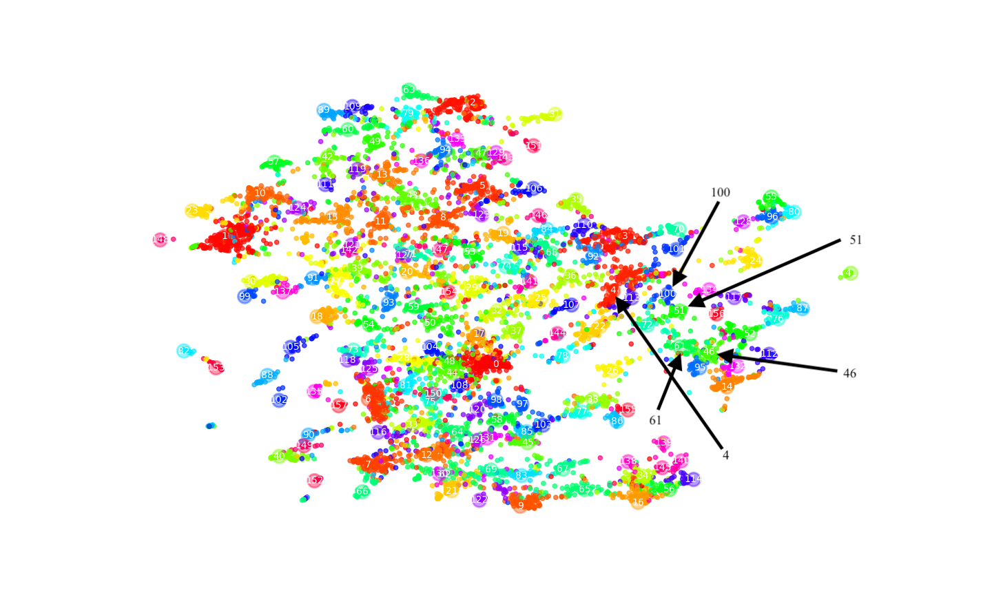
We can see towards the bottom right side of the plot that some of our key topics, 51, 100, 46, 4, are clustered in that quadrant of the graph. If we zero-in a bit we can see them laid out fairly “close” to one another:
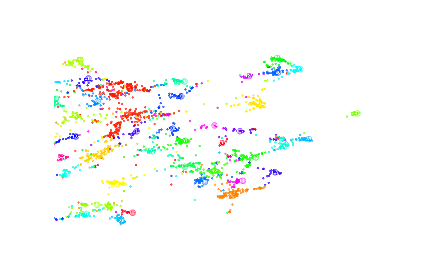
(For both images one can right-click ’em, open in a new tab and then zoom in—I’ll have to see if I can find a nice HUGO shortcode that would do this without having to load the image in a new tab …—I know there is some talk out there of potentially implmenting a Medium.com like zoom on images too.)
I would say that after all of the model building is completed (which, again, did take quite a while given the rather large size of our dataset), the steps needed are super quick and simple—and the ease with which all of this happens after model building is nothing short of really awesome. I am greatly looking forward to playing around with this library on all kinds of different datasets, that’s for sure! (As Dr. Mattingly noted in his second video, there are some parameters in Top2Vec [specifically the “speed” and “workers” ones] that could potentially speed up different parts of the process) that I should tweak and play around with a little bit to see what the effects are in the final visualizations and clustering of topics. More to come on this front, to be sure!
digital humanities machine learning supervised machine learning matplotlib data visualization work stuff python python for digital humanities pandas topic modeling Top2Vec united states supreme court opinions ussc
1370 Words
2022-07-07 00:13