General Background

(All code from this section is available in this repository here.)

Friday of last week, June 24th, 2022, was a profoundly dark day for a great many of us in the United States. Feeling somewhat helpless as the Supreme Court published the final draft of Dobbs v. Jackson Women’s Health Organization, I couldn’t help but fall back on old patterns. Not really knowing what else to do—I had a student with whom I had recently read the leaked original draft posted by Politico—I couldn’t help but say to her when the opinion came down that I didn’t know what else to do other than to get to reading. There’s something about the academic position—“Well, let’s get started reading …"—that felt so weak to me at the moment in the face of all the implications and consequences of this huge decision, but, honestly, I wasn’t quite sure what else to do other than to go to the default thing that the academic does: read … and think. Last Friday was a very dark day for sure; as I heard one commentator say (who exactly escapes me at the moment), it isn’t every day that you can wake up and can see that your daughter literally has fewer rights on that day than her own mother or grandmother had over all the decades since 1973. “A dark day” doesn’t even really capture things.

I read the draft decision multiple times—twice, in fact (or was it a f three times?)—; I read the finalized version of the opinion along with the concurring and dissenting opinions, again, twice. I figured this might be as good an opportunity as any to try out some of the things I’ve learned recently working with the whole topic modeling area of NLP and machine learning in general.

Roe v. Wade (410 US 113) Topic Modeling Over Time

Humanities Data Analysis: Case Studies with Python by Folgert Karsdorp, Mike Kestemont, and Allen Riddell (a fantastically awesome text, by the way, I should say!) has an entire chapter that would seem perfectly fine for our purposes here. Chapter 9, “A Topic Model of United States Supreme Court Opinions, 1900-2000,” has a ton of the data that we would want to be looking at here with regards to thinking about the Dobbs decision. Karsdorp, et. al. has a dataset with a .jsonl file with a ton of Supreme Court opinions separated by author name, case_id, the type of opinion, and the year the opinion was submitted. We start with the standard moves: importing the necessary libraries and getting the .jsonl file read into a dataframe:

import os
import gzip
import pandas as pd
import numpy as np
import matplotlib.pyplot as plt

with gzip.open('../datasets/supreme-court-opinions-by-author.jsonl.gz', 'rt') as fh:
    df = pd.read_json(fh, lines=True).set_index(['us_reports_citation', 'authors'])

We’re interested in looking at the Roe case, which is denoted as “410 US 113,” Harry Blackmun wrote the main opinion:

print(df.loc['410 US 113'].loc['blackmun', 'text'][:250])

OPINION BY: BLACKMUN
OPINION
MR. JUSTICE BLACKMUN delivered the opinion of the Court.
This Texas federal appeal and its Georgia companion, Doe v. Bolton, post, p. 179, present constitutional challenges to state criminal abortion legislation. The Tex

We can also just quickly looking at the distribution of opinions over time in the dataset if we like:

df['year'].hist(bins=50)

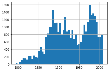
We can also get some simple information (how many opinions are there in the dataframe, etc.):

df['year'].describe()

    count    34677.000000
    mean      1928.824552
    std         48.821262
    min       1794.000000
    25%       1890.000000
    50%       1927.000000
    75%       1974.000000
    max       2008.000000
    Name: year, dtype: float64

The next thing we need to do is convert all of the text of each case’s opinion into a numerical representation that the computer can understand:

import sklearn.feature_extraction.text as text

vec= text.CountVectorizer(lowercase=True, min_df=100, stop_words='english')
dtm = vec.fit_transform(df['text'])

print(f'Shape of document-term matrix: {dtm.shape}. '
     f'Number of tokens: {dtm.sum()}')

This results in a (34677, 13231) matrix with a total number of tokens of 36,139,890—quite a few tokens there, to be sure. We then utilize the Latent Dirichlet Allocation model to transform the document-term matrix and find all the different “topics” contained within all our texts:

import sklearn.decomposition as decomposition
model = decomposition.LatentDirichletAllocation(n_components=100, learning_method='online', random_state=1)

document_topic_distributions = model.fit_transform(dtm)
vocabulary = vec.get_feature_names()
assert model.components_.shape == (100, len(vocabulary))
assert document_topic_distributions.shape == (dtm.shape[0], 100)

We can then have a look at the topic distributions that describe the case and Blackmun’s opinion. The result shows us that “Topic 14” is the highest:

blackmun_opinion = document_topic_distributions.loc['410 US 113'].loc['blackmun']
blackmun_opinion.sort_values(ascending=False).head(10)

Topic 14    0.261380
Topic 63    0.103755
Topic 6     0.079996
Topic 49    0.079675
Topic 17    0.049497
Topic 35    0.038979
Topic 42    0.037718
Topic 93    0.034306
Topic 78    0.033144
Topic 41    0.032153
Name: blackmun, dtype: float64

We can next look at the most frequently occuring words per this particular topic and it would seem to give us what we would expect:

topic_word_distributions.loc['Topic 14'].sort_values(ascending=False).head(18)

child        7148.398106
children     5668.526880
medical      5167.666624
health       3431.308011
women        3194.024162
treatment    2919.207243
care         2912.593764
hospital     2839.550152
family       2722.583008
age          2686.429177
parents      2646.981270
mental       2515.309043
abortion     2473.571781
social       2115.088729
statute      2025.966412
life         1893.954525
woman        1820.462268
physician    1813.155061
Name: Topic 14, dtype: float64

Karsdorp, et. al. next utilize the “Spaeth Issue Areas” (documentation for this is available through Washington University in St. Louis’s SCDB [“Supreme Court Database”]) that categorizes decisions based on a number of “broad areas”:

Values:
1 Criminal Procedure
2 Civil Rights
3 First Amendment
4 Due Process
5 Privacy
6 Attorneys
7 Unions
8 Economic Activity
9 Judicial Power
10 Federalism
11 Interstate Relations
12 Federal Taxation
13 Miscellaneous
14 Private Action

(# 14 was added since the 2016 version utilized in Karsdorp, et. al., so I have added it here.)First we put this into a dictionary; next we read in a dataframe the scdb_2021_case_based.csv file (also pulled from Wash U’s website) and then join this dataframe to our previous one containing all the opinions, being sure to join it together using the “issueArea” column from the SCDB file with the “case_id” column of the original opinions dataframe; lastly we utilize the pandas Categorical function to convert our wanted column to the Categorical datatype. We can then see how many of the opinions in our original dataframe fall under each of the different Spaeth areas within Topic 14:

issueArea
Criminal Procedure       33288.010972
Civil Rights            172757.834085
First Amendment          34239.879011
Due Process              33358.340810
Privacy                  93654.682271
Attorneys                 3454.198377
Unions                    3553.985849
Economic Activity        18875.924499
Judicial Power           23458.627270
Federalism               16451.143912
Interstate Relations        78.270460
Federal Taxation          2052.147267
Miscellaneous              526.598339
Private Action              20.014372
Name: Topic 14, dtype: float64

Curiously we see some rather high numbers for Topic 14 regarding the areas of “Civil Rights” and also the concern about “Privacy,” which should strike anyone and everyone that read the dissenting Dobbs opinion by Justices Breyer, Sotomayor, and Kagan as absolutely, positively spot-on (their dissent begins on page 148 of the .pdf copy here). A great deal of disagreement was about questions and concerns about “privacy”—the LDA model manages to pick that up quite, quite well: “Civil Rights” and “Privacy” are the key Spaeth areas for this topic—again, seems spot-on.

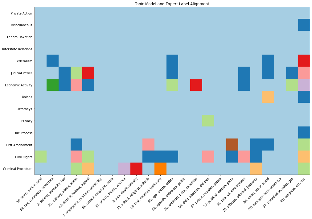
Karsdorp, et. al. also have a nice little heatmap that “[shows] the co-occurrence of topics and labels” (p. 309). They note that:

[f]or the most part, topics and Spaeth labels co-occur in an expected pattern. Topics which are associated with criminal procedure tend to co-occur with the Spaeth Criminal Procedure label. Topics associated with economic activity … tend to co-occur with the Economic Activity label. (p. 309)

For a redone version of that heatmap with a different color pallette is done with this code block:

fig, ax = plt.subplots()
im = ax.imshow(np.flipud(df_plot.values), cmap='Paired')
ax.set_xticks(np.arange(len(df_plot.columns)))
ax.set_yticks(np.arange(len(df_plot.index)))
ax.set_xticklabels(df_plot.columns)
ax.set_yticklabels(reversed(df_plot.index))
plt.setp(
    ax.get_xticklabels(), rotation=45, ha='right', rotation_mode='anchor')
ax.set_title('Topic Model and Expert Label Alignment')
)

which produces the following plot:

So we have all the data here wrangled together to start searching through some of these topics. Let’s say we wanted to zero-in on another key abortion case? Using some cataloging work from Pew Research, we could have a look at Webster v. Reproductive Health Svcs. (“492 US 490”)—with the opinion authored by Justice Rehnquist—from 1989? Then, we could include a keyword to search for—let’s try something like the word “viable.”

opinion_of_interest = ('492 US 490', 'rehnquist')
document_topic_distributions.loc[opinion_of_interest, viable_top_topics.index]

Curious—what if we took a look at the Stenberg v. Carhart (“530 US 914”) case from back in 2000?

opinion_of_interest = ('530 US 914', "breyer")
print(df.loc[opinion_of_interest, 'text'].values[0][0:1000])
print(
    f'"viable count in 530 US 914:',
    sum('viable' in word.lower()
       for word in df.loc[opinion_of_interest, 'text'].values[0].split()))
    
    OPINION BY: BREYER
    OPINION
    JUSTICE BREYER delivered the opinion of the Court.
    We again consider the right to an abortion. We understand the controversial nature of the problem. Millions of Americans believe that life begins at conception and consequently that an abortion is akin to causing the death of an innocent child; they recoil at the thought of a law that would permit it. Other millions fear that a law that forbids abortion would condemn many American women to lives that lack dignity, depriving them of equal liberty and leading those with least resources to undergo illegal abortions with the attendant risks of death and suffering. Taking account of these virtually irreconcilable points of view, aware that constitutional law must govern a society whose different members sincerely hold directly opposing views, and considering the matter in light of the Constitution's guarantees of fundamental individual liberty, this Court, in the course of a generation, has determined and then re
    "viable" count in 530 US 914: 3

And what if we wanted to look at these topic distributions over time? Are there any trends (increases in the frequency of our top topic words occuring over time, say) here that we might be able to see? Excellent question—and easy enough to do with a little coding; let’s see what we can see! So let’s figure out if we can’t “graph” Topic 14 and plot it over time.

topic_fourteen = 'Topic 14'
topic_word_distributions.loc[topic_fourteen].sort_values(ascending=False).head(10)

topic_top_words = topic_word_distributions.loc[topic_fourteen].sort_values(ascending=False).head(10).index
topic_top_words_joined = ', '.join(topic_top_words)
print(topic_top_words_joined)

  child, children, medical, health, women, treatment, care, hospital, family, age

Next we’ll count up how many times these top topic words appear (as a proportion of the total words written in a particular year) in our document_topic_distributions matrix:

opinion_word_counts = np.array(dtm.sum(axis=1)).ravel()
word_counts_by_year = pd.Series(opinion_word_counts).groupby(df.year.values).sum()
topic_word_counts = document_topic_distributions.multiply(opinion_word_counts, axis='index')
topic_word_counts_by_year = topic_word_counts.groupby(df.year.values).sum()
topic_proportion_by_year = topic_word_counts_by_year.divide(word_counts_by_year, axis='index')
topic_proportion_by_year.head()

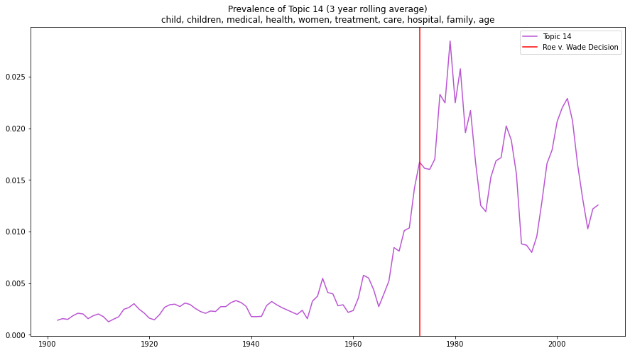
I’ll save the printout of the dataframe’s head and just go to the visualization, which looks like this (the red vertical line marks the year Roe was decided, 1973), utilizing the following code:

plt.figure(figsize=(15, 8))
window = 3 
topic_proportion_rolling = topic_proportion_by_year.loc[1900:, topic_fourteen].rolling(window=window).mean()
topic_proportion_rolling.plot(color='mediumorchid')
plt.title(f'Prevalence of {topic_fourteen} ({window} year rolling average)'
          f'\n{topic_top_words_joined}')
plt.axvline(x=1973, color='red', label="Roe v. Wade Decision")

(We could easily get the counts of the word “abortion” instead if we so wanted.)

plt.figure(figsize=(15, 8))
abortion_top_topics = topic_word_distributions['abortion'].sort_values(ascending=False).head(5)
abortion_top_topics_top_words = topic_word_distributions.loc[abortion_top_topics.index].apply(lambda row: ', '.join(row.sort_values(ascending=False).head().index), axis=1)
abortion_top_topics_top_words.name = 'topic_top_words'

opinion_of_interest_1 = ('492 US 490', "rehnquist")
print(
    f'"abortion" count in 492 US 490:',
    sum('abortion' in word.lower()
       for word in df.loc[opinion_of_interest_1, 'text'].values[0].split()))

document_topic_distributions.loc[opinion_of_interest_1, abortion_top_topics.index]

(It would be nice to rewrite some of these explorations into a function that we could easily just call in a single line [a task for another day, I would bet]). In terms of conclusions one might draw here—especially the graph showing the rolling 3-year window, one could easily say that a marked increase in documents showing a concern with topics surrounding women, medical care, abortion, viability, and other connected ideas (“child and children,” “care”, “hospital,” “family,” and so on) occur right around the time of the Roe decision. Of course, I would want to suggest that the plots above are a perfectly empirical, “data-driven” way to talk about the United States’s history with regards to women and their concerns. The main opinion from Justice Alito talked a big game about the use of a proper historical understanding of the whole “abortion” issue. Another part of that history, too, of course, is a quite profound lack of interest in women’s equality. That too, sadly to say, is also a part of this whole “history” and for many of us what the Dobbs decision did was, unfortunately, to simply continue that larger trend of disregard for women’s equality.

I was planning to show how the Top2Vec library) handles all of this, but this post is getting a bit on the long side; I was also hoping to post some stylometric analysis of three of the recently-new justices (Gorusch, Kavanaugh, and Barrett), but I’ll save that for yet another post. So, two more posts to come on this arena here in the near future.

(Nota bene: It would probably also be nice to update the .csv file/database with opinions that occurred after 2016, bringing them more up-to-date. I’ll see if I can write-up something about using the really fantastic Court Listener API to fetch the plain text of the opinions from the years between 2016 and 2022.)