Binary Text Classification Fun! … with some Literary Texts by Willa Cather and Sarah Orne Jewett

In my DH journey, the work of Dr. William Mattingly has been something of a constant companion and guide.

His video laying out the steps for a “Binary Data Classification” was clear and quite clarifying for me in all kinds of ways. The classifier’s job in this video was to see if it could tell the difference between the work of Oscar Wilde and Dan Brown. What if we tried a different pair of authors/texts? As I offhandedly mentioned in my previous post, finding texts in the public domain (like Shakespeare’s for example), saves one quite a bit of time wrangling things together. I also, for some, reason, have found myself going back to some of the works of Willa Cather (admittedly, she’s definitely not in my wheelhouse/field of study by any stretch of the imagination) and was wondering how a machine learning classifier might perform when looking at Cather’s texts alongside those of one of her key influences, Sarah Orne Jewett (image below is courtesy of UNL’s fantastic Willa Cather Archive here):

Why not?—I figured I could tinker around a bit to see what’s possible. Project Gutenberg has a number of texts by both Cather and Jewett—and the UNL Willa Cather Archive has a good number of her texts formatted in .xml. I grabbed as many of the texts as I could from these two sources. Since the Gutenberg texts come with the typical boilerplate material at the start and end of the plain text file I pulled out a nice little script from “C-W” on GitHub that had a nice list of phrases used in the boilerplate material; the simple script would strip all the boilerplate when the text files get read in.

The major steps here for this tinkering is to read in all the plain text files, split everything up by sentences, write a function that will “pad” the data so that any sentences that are less than a specific length ultimately get a ? added to the sentence to bring it’s length up to the already specified max_length of each sentence. This is due to the way that the keras library likes to have data fed to it. That function looks as follows:

def padding_data(sentences, index, maxlen=25):
    new_sentences = []
    for sentence in sentences:
        sentence = text_to_word_sequence(sentence)
        new_sentence = []
        words = []
        for word in sentence:
            try:
                word = index[word]
            except:
                KeyError
                word = 0
            words.append(word)
        new_sentence.append(words)
        new_sentence = preprocessing.sequence.pad_sequences(new_sentence, maxlen=maxlen, padding='post')
        new_sentences.append(new_sentence[0])
    return(new_sentences)

Next is a function that will index each and every token within the text file and append it to a .json file that will store every token and its associated index number:

def create_index(texts, filename):
    words = texts.split()
    tokenizer = Tokenizer(num_words = 100000)
    tokenizer.fit_on_texts(words)
    sequences = tokenizer.texts_to_sequences(words)
    word_index = tokenizer.word_index
    print(f"Found {len(word_index)} unique words.")
    with open(filename, "w") as f:
        json.dump(word_index, f, indent=4)

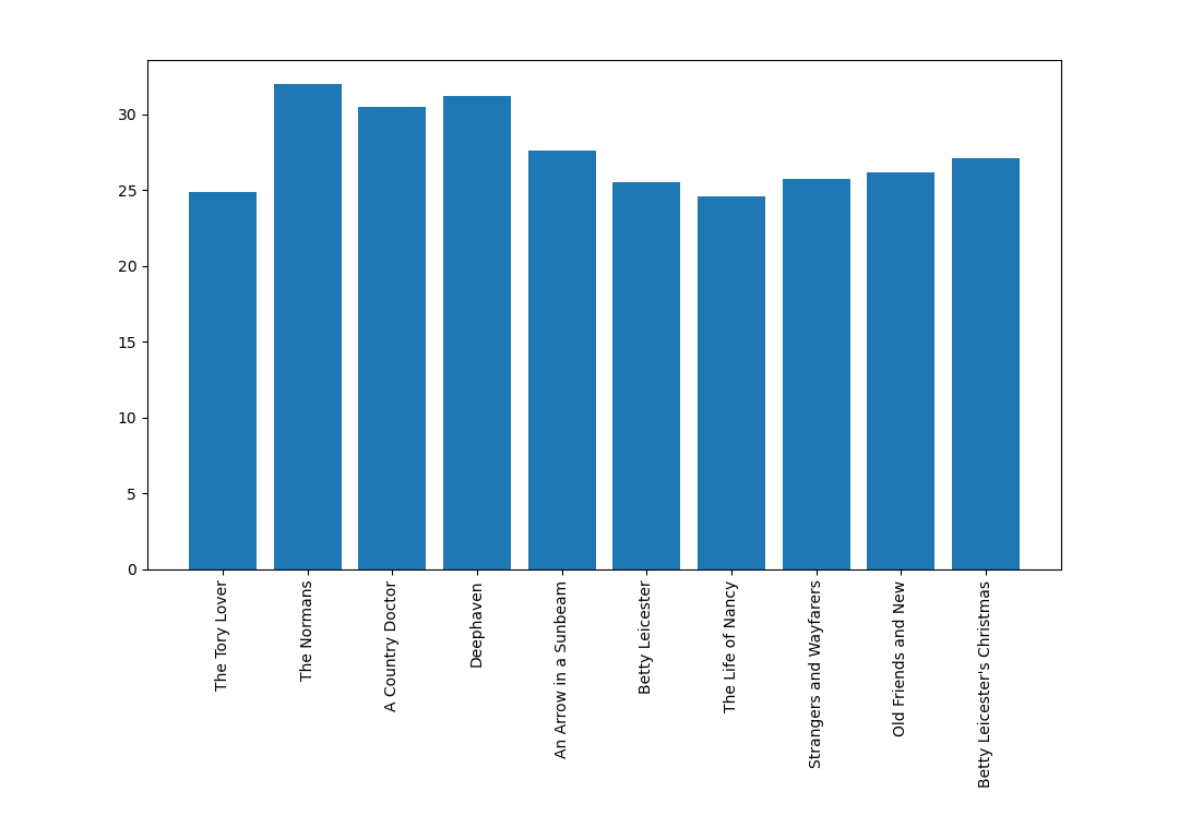
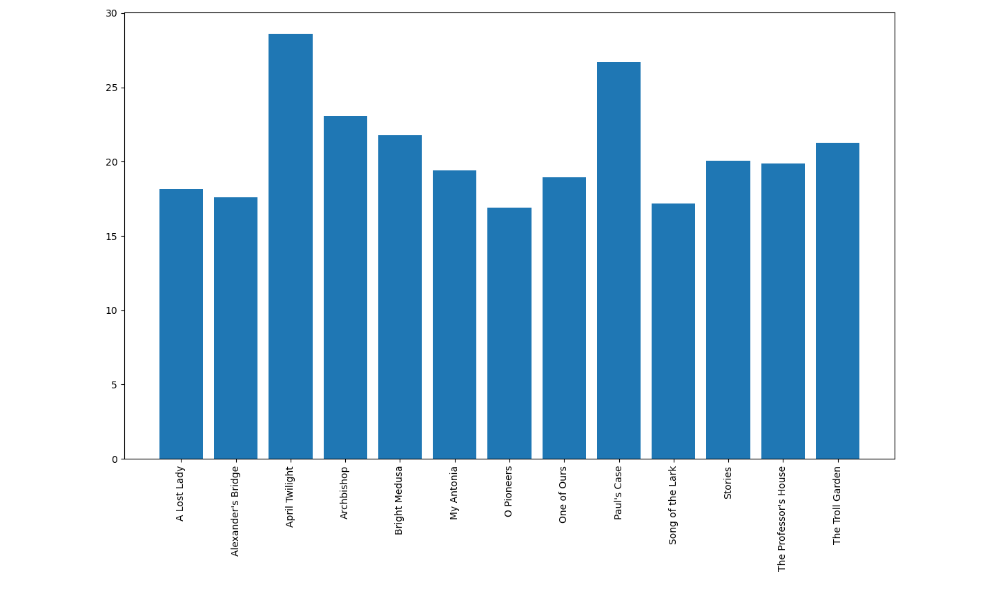
In the tutorial, Mattingly uses a max_length of 25 words; a quick graph of the average sentence lengths for each of our author’s texts would suggest that number is probably not a bad choice for our dataset:

We also need to label all of the sentences so we can keep all the sentences and words by Cather paired up together with all the sentences and words by Jewett:

def label_data(sentences, label):
    total_chunks = []
    for sentence in sentences:
        total_chunks.append((sentence, label))
    return(total_chunks)

Now with all the data structured and ordered in the way the keras model needs it, we can create the training data, create, train, and fit the model on the dataset:

def train_model(model, tt_data, val_size=.3, epochs=1, batch_size=16):
    vals = int(len(tt_data[0])*val_size)
    training_data = tt_data[0]
    training_labels = tt_data[1]
    testing_data = tt_data[2]
    testing_labels = tt_data[3]

    x_val = training_data[:vals]
    x_train = training_data[vals:]

    y_val = training_labels[:vals]
    y_train = training_labels[vals:]

    fitModel = model.fit(x_train, y_train, epochs=epochs, batch_size=batch_size, validation_data=(x_val, y_val), verbose=2, shuffle=True)
    print(fitModel.history.keys())
    import matplotlib.pyplot as plt
    plt.plot(fitModel.history['loss'])
    plt.plot(fitModel.history['val_loss'])
    plt.title('model loss')
    plt.ylabel('loss')
    plt.xlabel('epoch')
    plt.legend(['train', 'test'], loc='upper left')
    plt.show()
    plt.clf()
    plt.plot(fitModel.history['accuracy'])
    plt.plot(fitModel.history['val_accuracy'])
    plt.title('Model accuracy')
    plt.ylabel('Accuracy')
    plt.xlabel('Epoch')
    plt.legend(['Train', 'Val'], loc='lower right')
    plt.show()
    model_results = model.evaluate(testing_data, testing_labels)
    return(model)

After testing, the loss and accuracy for the model turned out to be [0.32046514101210954, 0.875969] respectively. The keras library also allows us to see the loss and accuracy over each epoch of training:

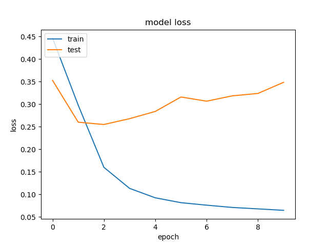
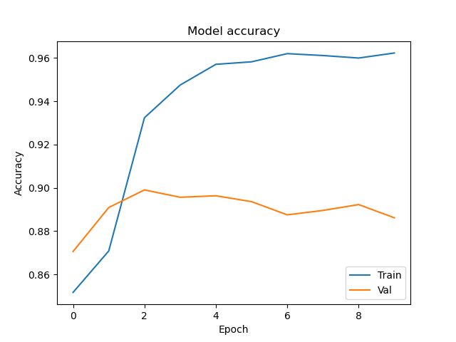
In the code snippet above the plot was included in the train_model function, but one could just as easily pull them out as their own functions so we have one function only do one specific job.

def plot_model_loss(model_name, string_1='loss', string_2='val_loss'):
    plt.plot(model_name.history[string_1])
    plt.plot(model_name.history[string_2])
    plt.title('model loss')
    plt.ylabel(string_1)
    plt.xlabel('epoch')
    plt.legend(['train', 'test'], loc='upper left')
    plt.show()

def plot_model_accuracy(model_name, string_1='accuracy', string_2='val_accuracy'):
    plt.plot(model_name.history[string_1])
    plt.plot(model_name.history[string_2])
    plt.title('model accuracy')
    plt.ylabel('accuracy')
    plt.xlabel('epoch')
    plt.legend(['train', 'val'], loc='lower right')
    plt.show()

What happens when we turn the model on a text by, say, Cather, that it has not seen yet before? I quite enjoy her short story, “Paul’s Case: A Study in Temperament.” The script will read in the text, utilize the word_index.json file to replace each word with the number of that word in the index. One can then keep track of each sentence to see the model’s predictions: a score close to 0 suggests the model thinks it’s by Cather; the closer to 1, the prediction is that it belongs to Jewett. (The full test log file from the console is available here.) We could easily write a little bit of code as well to get the .txt file with all the predictions into a DataFrame for even further analysis; it’s relatively quick and simple to get some nice scatter plots of the predictions for each and every sentence in the story:

import pandas as pd
import matplotlib.pyplot as plt

file = r'cather_jewett\interpreting_model_results\mate_of_the_daylight_results.txt'
results = pd.read_csv(file, header=None, sep=',')
results.rename(columns={0: 'prediction', 1: 'text'}, inplace=True)
results['test'] = results['prediction'].str.extract(r'((?<=\[).*?(?=\]))')
results['cleaned_prediction'] = results['test'].astype(float)
cather_df = results.loc[results.cleaned_prediction <= 0.5]
jewett_df = results.loc[results.cleaned_prediction >= 0.5]
predictions = results['cleaned_prediction']
plt.plot(predictions)
plt.clf()
plt.scatter(predictions.index, predictions.values, alpha=0.4, color='firebrick')
plt.xlabel("sentence")
plt.ylabel("prediction")
plt.title("Predictions for Each Sentence of Cather's 'Paul's Case'")
plt.show()

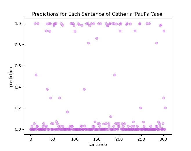
Most of the sentences are predicted to be by Cather. Curiously, feeding the model a text by Jewett, “A Mate of the Daylight,” most of the predictions are towards the Cather side of the graph:

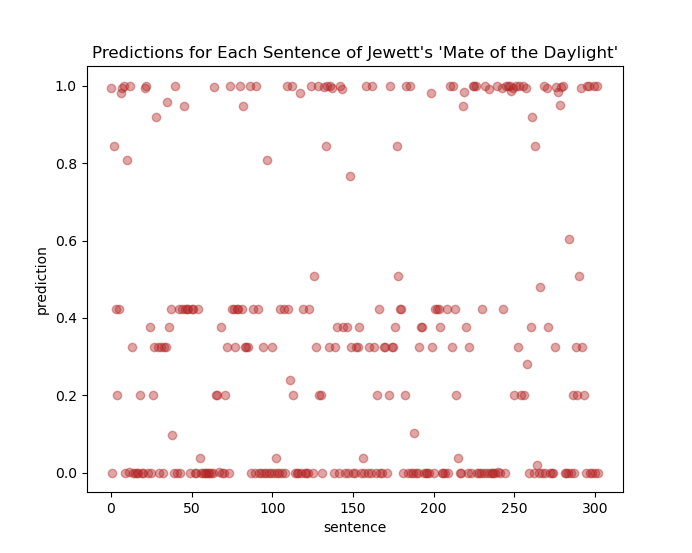
It would no doubt be good to do a little bit of digging here to see what might be going on with the model’s predictions about this Jewett story. Also, hopefully, in the near future, I can do a little bit of writing about some of the other classifiers one could build and set to work on these Cather and Jewett texts.

Again, as usual, more to come …