Using Vector Space Models with Shakespeare’s Plays

Much of the toe-dipping into this new DH field I’ve been doing as of late has centered around learning many of the kinds of projects carried out and then turning the methods within those projects onto mew artifacts. A while back I worked my way through Folgert Karsdorp, Mike Kestemont, and Allen Riddell’s Humanities Data Analysis: Case Studies with Python. I found a great deal of it thought-provoking and fascinating—especially the chapters devoted to modeling texts with vector spaces and the later chapter on stylometry, which focused on some texts by Hildegard of Bingen and Bernard of Clairvaux. With regards to the first vector space angle, a good deal of very old and dusty linear algebra from my undergraduate days has been rattling around in my head as of late—and it was quite fun to see if I could get any of the old gears turning again (some I definitely could, others will need a bit more grease to get things moving once more).

Chapter 3 of Humanities Data Analysis focused on visually “mapping” a number of different genres of plays from classical French theater, utilizing some vector space math. I wondered what things would look like if we turned these methods on some of Shakespeare’s works. All the plays Karsdorp, et. al. were working with were in .xml format—and after learning how much time the data analyst working on just getting data into a form and structure (“preprocessing” that is ready for analytic work in the first place, it seemed easy enough to simply grab the bard’s texts from The Folger Shakespeare, especially since one can get them all in TEI Simple .xml format—which makes all the plays incredibly easy to parse since all the work of encoding has been done for one already. As most readers of Shakespeare know, his work has often been carved up into similar genres categories to the one’s Karsdorp, et. al. were using on their French theater corpus—i.e. into comedies, tragedies, tragicomedy, etc. So I figured I could try something similar with this different corpus.

After grabbing the TEI texts from Folger, we could get some libraries imported and then create some lists with genres and the plays that belong to those genres (it’s a little rough, but I simply used the age-old “comedy/history/tragedy/late romance” categories).

comedies = [
    "All’s Well That Ends Well",
    "As You Like It",
    "The Comedy of Errors",
    "Love’s Labor’s Lost",
    "Measure for Measure",
    "The Merchant of Venice",
    "The Merry Wives of Windsor",
    "A Midsummer Night’s Dream",
    "Much Ado About Nothing",
    "The Taming of the Shrew",
    "Twelfth Night",
    "Two Gentlemen of Verona"
    ]
histories = [
    'Henry IV, Part I',
    'Henry IV, Part II',
    'Henry V',
    'Henry VI, Part 1',
    'Henry VI, Part 2',
    'Henry VI, Part 3',
    'Henry VIII',
    'King John',
    'Richard II',
    'Richard III'
    ]
tragedies = [
    'Antony and Cleopatra',
    'Coriolanus',
    'Hamlet',
    'Julius Caesar',
    'King Lear',
    'Macbeth',
    'Othello',
    'Romeo and Juliet',
    'Timon of Athens',
    'Titus Andronicus',
    'Troilus and Cressida'
    ]
late_romances = [
    'Pericles',
    "The Winter's Tale",
    "The Tempest",
    'Cymbeline'
    ]

Next we create some empty lists to keep track of the title of the play, the genre it’s in, and then the actual text of the play—in creating the last one we’ll also grab all the words from each of the plays using the lxml library to get all of the words in the plays.

file_directory = glob.glob('./plays/*.xml')
plays, titles, genres = [], [], []

# let's loop through the texts, parse the XML and grab all the words in each play, etc.
for f in file_directory:
    parser = etree.XMLParser(collect_ids=False)
    tree = etree.parse(f, parser)
    xml = tree.getroot()

    # Now let's grab all the w ("word") tags in each play
    word_tags = xml.findall(".//{*}w")
    #title = xml.find(".//tei:titleStmt//tei:title", namespaces=nsmap).text
    title = xml.find(".//tei:teiHeader//tei:fileDesc//tei:titleStmt//tei:title", namespaces=nsmap).text
    #title = tree.find(".//tei:titleStmt//tei:title", namespaces=nsmap).text
    if title in comedies:
        genres.append('Comedies')
        titles.append(title)
        words = [word.get('reg', word.text).lower() for word in word_tags if word.text != None]
        plays.append(words)
    elif title in histories:
        genres.append('Histories')
        titles.append(title)
        words = [word.get('reg', word.text).lower() for word in word_tags if word.text != None]
        plays.append(words)
    elif title in tragedies:
        genres.append('Tragedies')
        titles.append(title)
        words = [word.get('reg', word.text).lower() for word in word_tags if word.text != None]
        plays.append(words)
    elif title in late_romances:
        genres.append('Late Romances')
        titles.append(title)
        words = [word.get('reg', word.text).lower() for word in word_tags if word.text != None]
        plays.append(words)

Now we have our three lists with all the information we’ll need moving forward. Karsdorp, et. al. then write a couple of functions here to generate a vocabulary from the texts along with a “document-term matrix”:

def extract_vocabulary(tokenized_corpus, min_count=1, max_count=float('inf')):
    vocabulary = collections.Counter()
    for document in tokenized_corpus:
        vocabulary.update(document)
    vocabulary = {
        word for word, count in vocabulary.items()
        if count >= min_count and count <= max_count
    }
    return sorted(vocabulary)

def corpus2tdm(tokenized_corpus, vocabulary):
    document_term_matrix = []
    for document in tokenized_corpus:
        document_counts = collections.Counter(document)
        row = [document_counts[word] for word in vocabulary]
        document_term_matrix.append(row)
    return document_term_matrix

Karsdorp, et. al., following Schöch, use a couple of French words (monsieur and sang) that are thought to have “considerable discriminative power for these genres.”¹ When we call the two functions above on our plays list, we get: document term matrix with |D| = 37 documents and |V| = 15733 words.

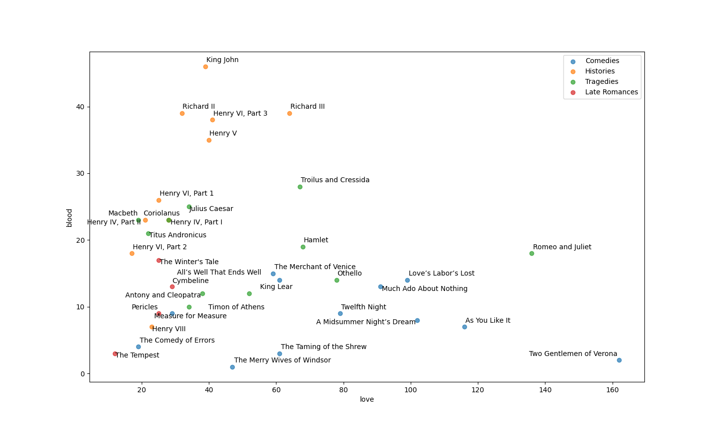
With all of this in a numpy array, it’s simple enough to look up a word in the matrix, find it’s index, and then see how all of the plays/genres use that word. What if we used the English “blood” and “love” to map out all of the plays/genres? We’d get something like the following:

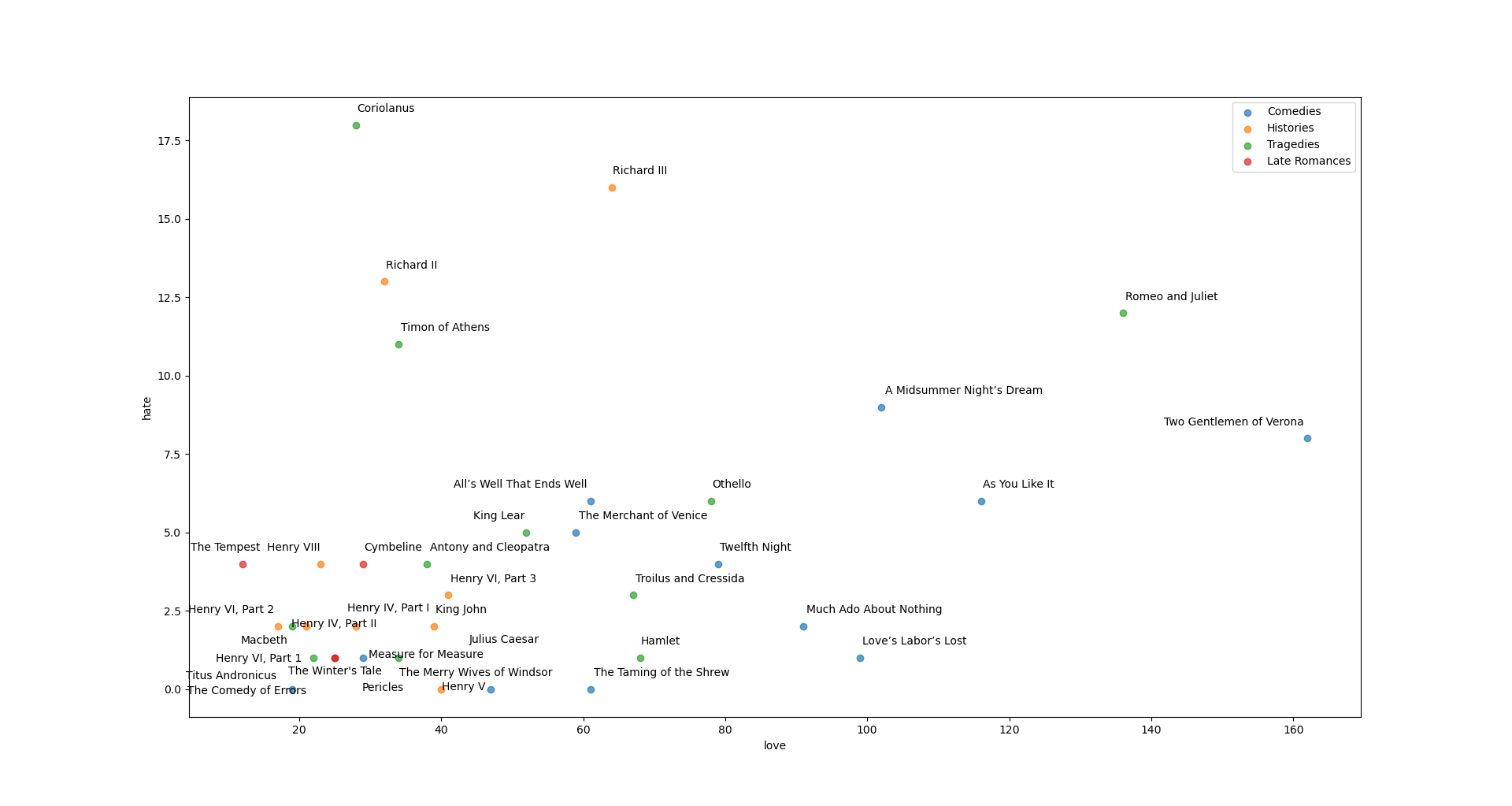
We could substitute any other word we like and then see how “close” together the plays are when focusing on the two words of our choosing—here’s “love” and “hate” on the X and Y axis respectively (the repo for all of this also has functions that will allow one to use different “distance metrics” with which to define and quantify the “closeness” or “similarity’ between any two plays or between different genres”):

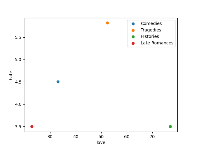
We could also wonder a bit about how the genres themselves get arranged—simple enough:

I suppose what I’ve found most useful here is not so much any profound insights into the bard’s works (it’s great to find other (computation/visual/digital) ways into his texts—and often for me that can function as a nice result in and of itself, but, instead, this “computational” way of thinking about things that is no doubt still really new and foreign to my strictly humanities-oriented background and training. It’s incredibly simple, but learning how to get all of these plays into a nice, structured format that one can then write a couple of rather simple functions to then produce visualizations of the data that are another avenue into the original texts is really fantastic. Not to mention the fact that one could then take these very simple functions/calculations and utilize them in different situations—say, for example, using them in a machine learning algorithm for authorship attribution or in larger projects within the realm of stylometry, etc.—has made all this new knowledge and all these new skills incredibly generative. (With regards to Shakespeare’s “late romances”—my mentor in graduate school just called them tragicomedies—I could imagine grabbing a bunch of texts by playwrights that would follow in the wake of Shakespeare: I have only recently come across the “EarlyPrint” website, which I know has a number of plays by Beaumont and Fletcher. It would be curious to see how close or far away those texts are from some of the plays within the “late romances” list above … )

As usual, more to come, for sure.