Viral Tweet Classification Project

I had a bit of fun recently working on a machine learning classification project using some Twitter data (said project coming through Codecademy). The goal was to see if we could write some code to properly detect whether or not a tweet was viral (using the K-Nearest Neighbors algorithm). I also played around with a logistic regression model as well. All the code for the following is available in this repo. I then took all this dabbling and turned the algorithms on some different datasets of a much more “literary” kind. (Another post is still to come on seeing how well the algorithms might be able to distinguish between Willa Cather and one of her key predecessors, Sarah Orne Jewett.)

So, first things first, we’re importing the necessary libraries for this task:

import matplotlib.pyplot as plt
from sklearn.preprocessing import scale
from sklearn.model_selection import train_test_split
from sklearn.neighbors import KNeighborsClassifier
import pandas as pd
pd.options.display.width = 0

After reading in all the Twitter data from a .json file, we needed to think a little bit about how exactly we might want to define a “viral tweet”? Base it solely on the number of retweets, on the number of likes, on the number of favorites? The parameters for the original task suggested we might start with the median number of retweets for each tweet (I also had a look at the favorite_count as well to see what the minimum, maximum, median, and mean numbers looked like):

retweet_counts = viral_tweets['retweet_count']
median_retweet_count = viral_tweets['retweet_count'].median()
mean_retweet_count = viral_tweets['retweet_count'].mean()

print(viral_tweets.agg(
    {
        "retweet_count": ["min", "max", "median", 'mean'],
        "favorite_count": ["min", "max", "median", "mean"],
    }
))

Graphing these values we get the following: 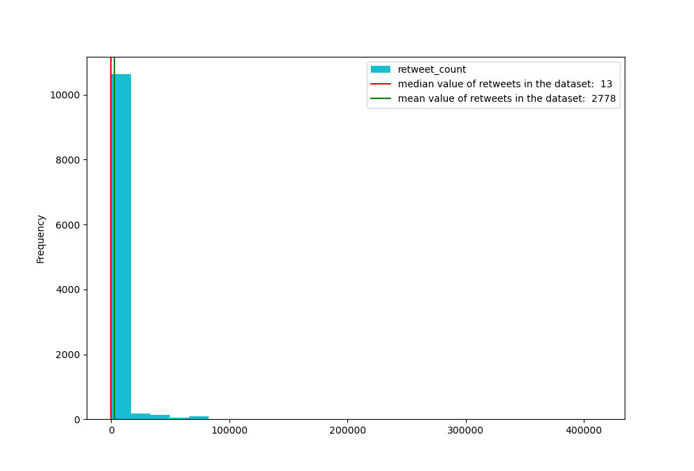The first time around here I just went with the median value as the cutoff for a “viral tweet,” so any row in the pandas dataframe that had more than the median number in a row, a new is_viral column got created and the row coded with 1 if it met the threshold and a 0 otherwise:

viral_tweets['is_viral'] = viral_tweets['retweet_count'].apply(lambda x: 1 if x > median_retweet_count else 0)

Next we started having a look at some of the other columns to see which ones might be helpful in predicting if a tweet would meet the median value threshold. Taking a look at the tweet_length, along with the numbers of followers and friends that a Twitter user had, we grabbed this data:

viral_tweets['tweet_length'] = viral_tweets.apply(lambda x: len(x['text']), axis=1)
viral_tweets['followers_count'] = viral_tweets.apply(lambda x: x['user']['followers_count'], axis=1)
viral_tweets['friends_count'] = viral_tweets.apply(lambda x: x['user']['friends_count'], axis=1)

Next we separated out the is_viral as that will contain the label of each tweet (1 for viral, otherwise 0). Next we dropped all the columns from the dataframe that we weren’t planning on using and just keeping the following list of columns: ['tweet_length', 'followers_count', 'friends_count']. We scaled the data, getting us ready to start separating out the training and testing data and then training and fitting the classifier/model to the training data.

As per usual, we used the train_test_split function from sklearn’s library:

train_data, test_data, train_labels, test_labels = train_test_split(scaled_df, labels, test_size = 0.2, random_state = 1)

classifier = KNeighborsClassifier(n_neighbors = 5)
classifier.fit(train_data, train_labels)
print(classifier.score(test_data, test_labels))

Next we wrote a short little loop to keep track of the classifier’s scores on the testing data using a different number of “clusters” (neighbors) ranging from 1 all the way up to 200

scores = []
for k in range(1, 200):
    classifier = KNeighborsClassifier(n_neighbors = k)
    classifier.fit(train_data, train_labels)
    scores.append(classifier.score(test_data, test_labels))
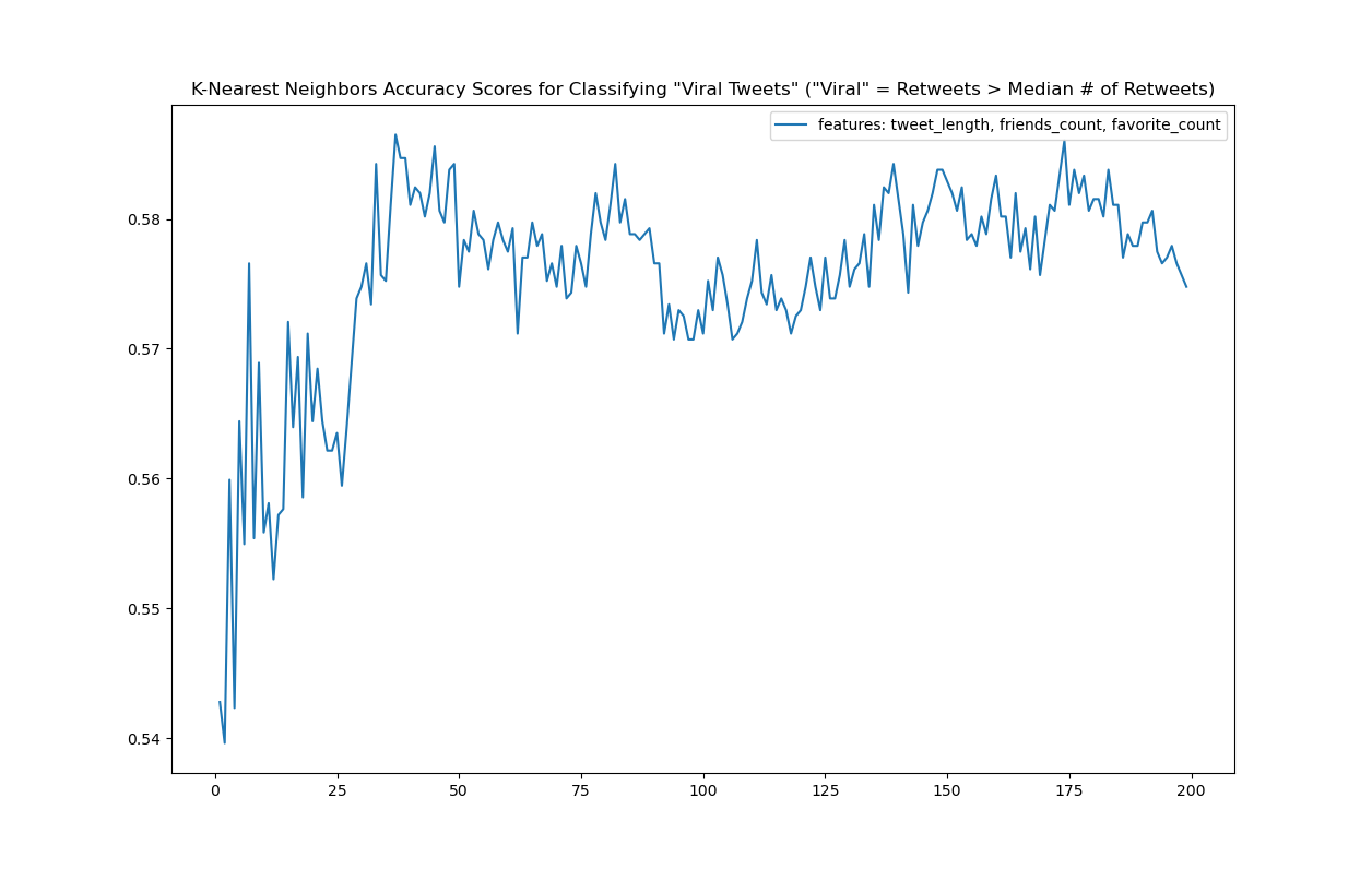
plt.plot(range(1,200), scores)
plt.legend(['features: tweet length, # of followers, # of friends'])

along with a graph:

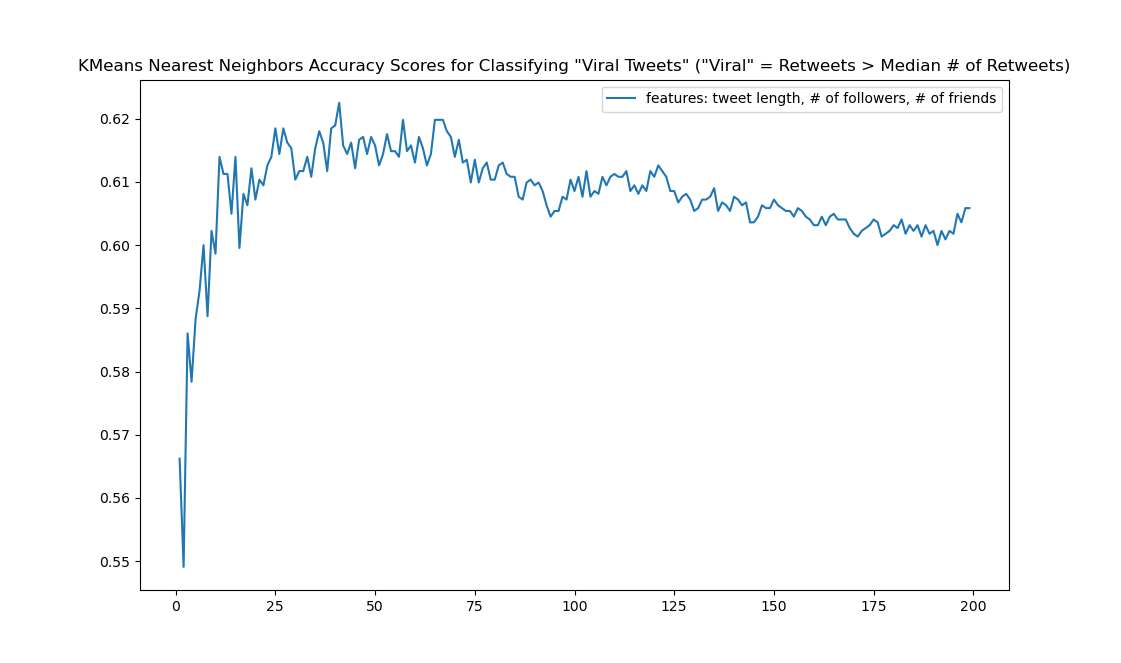
So we can see the roughly effectiveness of the classifier’s ability to detect a viral tweet (based only on the data in the 'tweet_length', 'followers_count', and 'friends_count' columns) hovering around 60% or so. There’s a steady drop off once the numbers of clusters gets to around 75.

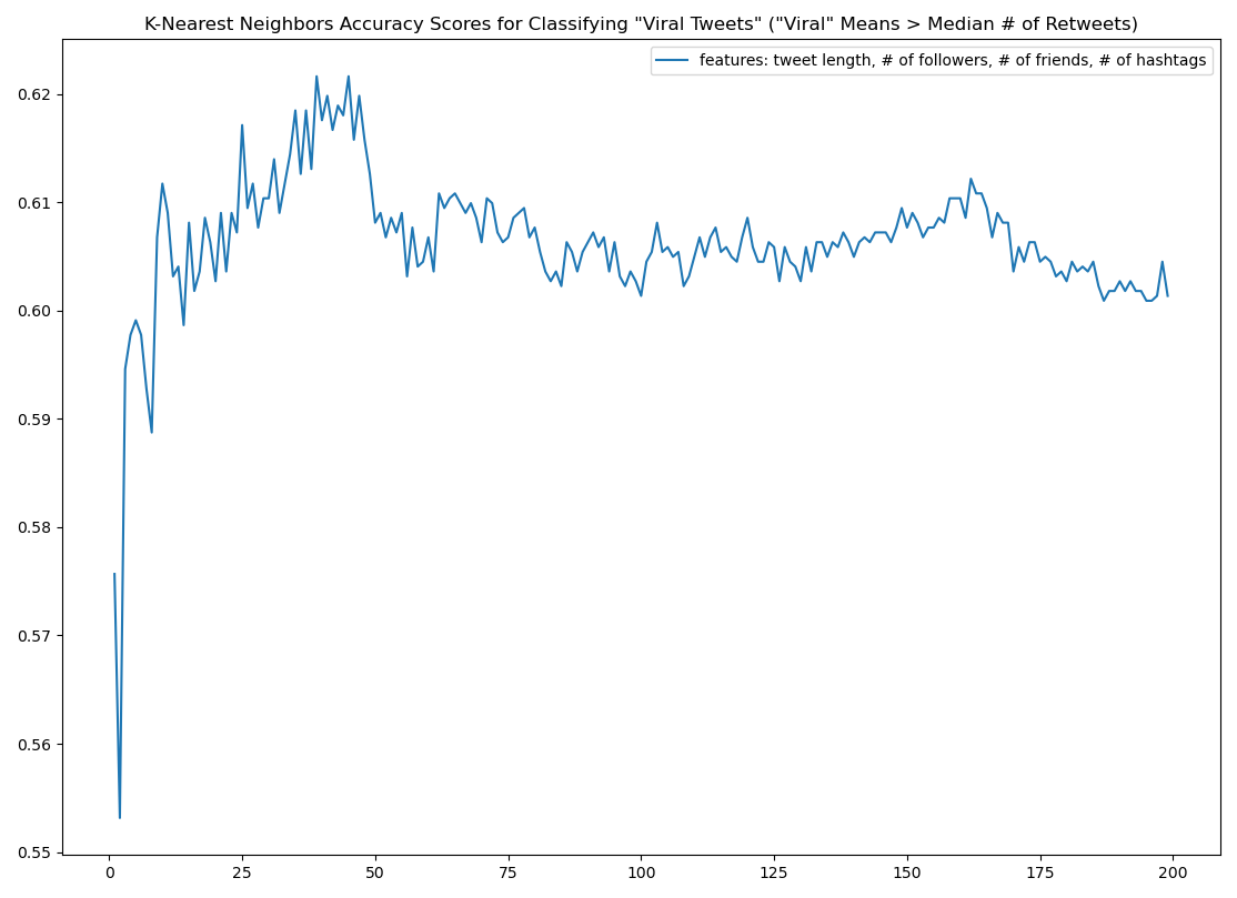
The project then wondered if there were other features within the dataset that we could use to increase the model’s predictive effectiveness. For this next round I added the 'number_of_hashtags' to see what results that might produce. We then added that column and retrained the classifier:

hashtag_col_added = ['tweet_length', 'followers_count', 'friends_count', 'number_of_hashtags']
hashtag_df = viral_tweets[hashtag_col_added]
scaled_hashtag_df = scale(hashtag_df, axis=0)
h_train_data, h_test_data, h_train_labels, h_test_labels = train_test_split(scaled_hashtag_df, labels, test_size=0.2, random_state=1)
classifier.fit(h_train_data, h_train_labels)
print(classifier.score(h_test_data, h_test_labels))

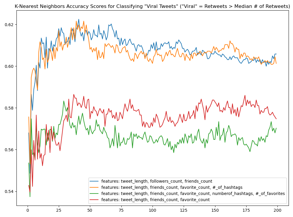
Scores taking the hashtags into account were as follows:

A model with the 'tweet_length_alone':

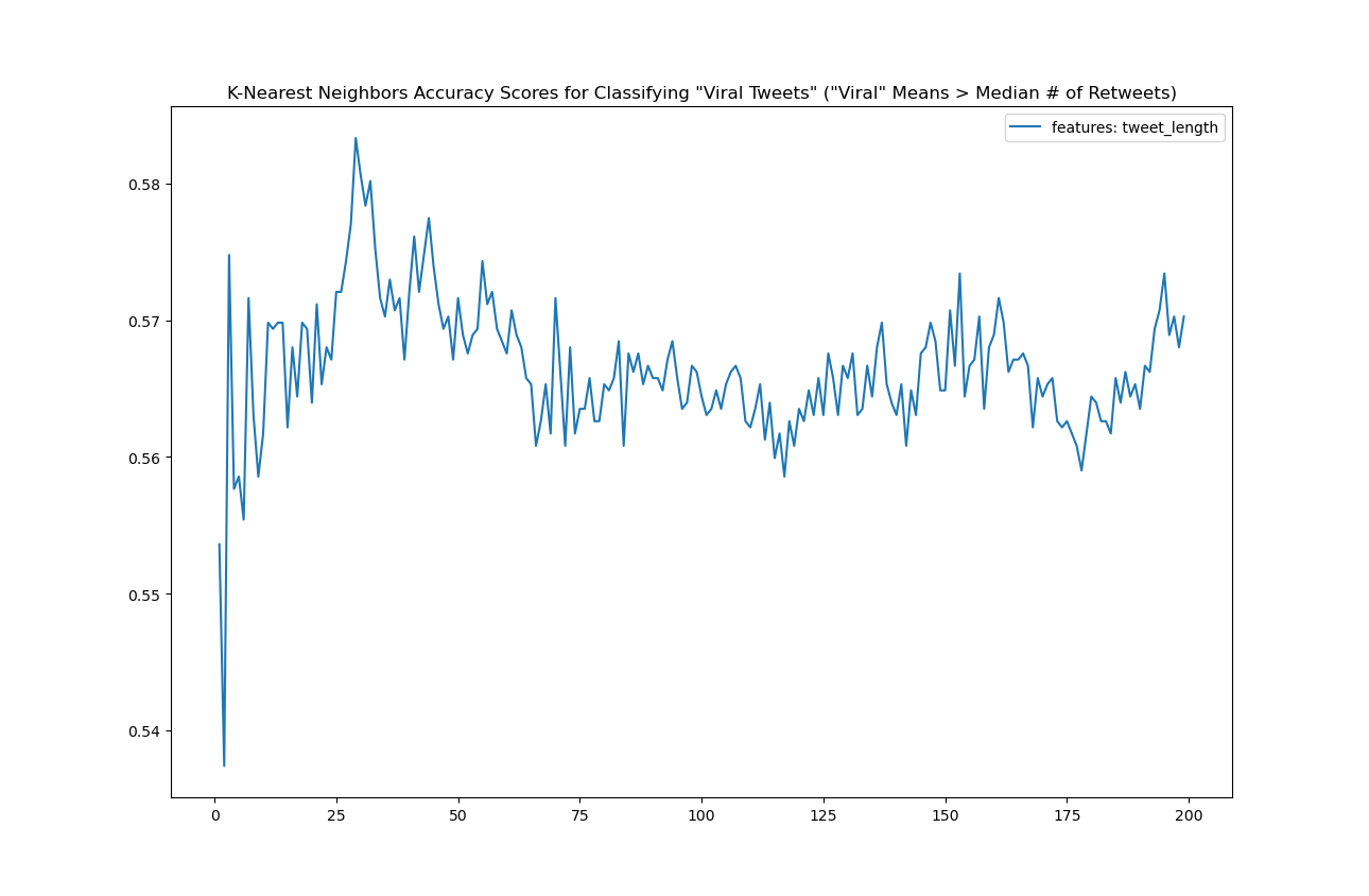
It was intriguing to continue to add features to the classifier to see what the results would be—it was easy enough to thus train multiple models (with different numbers of features) and graph their effectiveness. I tried models where we added 'favorite_count'.

Curiously, the model with the most features in it performed far less well than the ones with fewer:

One of the suggestions in the project asked one to wonder a bit about the threshold we used to define a “viral tweet.” We started with the median for the number of retweets a tweet in the dataset received. That number, 13, what if we tinkered a bit with that number? The mean for the 'retweet_count' was much higher. Would the classifier before any better if we set the threshold at the mean? Easy enough to have a look-see. Rerunning the script with the mean as the threshold, again splitting the dataset, training the models, and then plotting some scores, we get a considerable increase in accuracy: 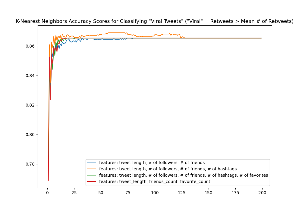All of these models—with varying numbers of features used—performed much better; all four of them level-out right around 86% accuracy, with the model utilizing “tweet_length, # of followers, # of friends, and # of hashtags” performing best amongst the four.

Super-fun stuff—to be sure.